


ABSTRACT
Parameters and abundances for 1133 stars of spectral types F, G, and K of luminosity class III have been derived. In terms of stellar parameters, the primary point of interest is the disagreement between gravities derived with masses determined from isochrones, and gravities determined from an ionization balance. This is not a new result per se, but the size of this sample emphasizes the severity of the problem. A variety of arguments led to the selection of the ionization-balance gravity as the working value. The derived abundances indicate that the giants in the solar region have Sun-like total abundances and abundance ratios. Stellar evolution indicators have also been investigated with the Li abundances and the [C/Fe] and C/O ratios, indicating that standard processing has been operating in these stars. The more salient result for stellar evolution is that the [C/Fe] data across the red-giant clump indicates the presence of mass-dependent mixing in accord with standard stellar evolution predictions.
Export citation and abstract BibTeX RIS
1. INTRODUCTION
This paper and its predecessors (Heiter & Luck 2003; Luck & Heiter 2005, 2006, 2007) are part of a program to examine the abundance properties of the local region in an effort to determine the standard of normalcy in terms of abundances. The intent on a very local scale—15 pc—is to examine in detail the abundance distribution in dwarfs. On a larger scale—out to 100 pc—the objective is to sample the volume using G/K giants as probes. The primary goal is an increased understanding of the local region about the Sun. The metallicity data should reveal whether there are any believable temporal, spatial, or stellar characteristic-related variations in the metallicity. If one considers the local region as a typical volume, then these results can be applied to other locations and thus will increase our understanding of galactic evolution. The hope that these studies will be useful in understanding chemical evolution has been borne out by subsequent studies of open clusters (Reddy et al. 2012, 2013), and an examination of carbon and oxygen abundances across the Hertzprung Gap (Adamczak & Lambert 2014), which used the results of Luck & Heiter (2007)—hereafter LH07—as a comparison benchmark. In LH07, the examination of trends in carbon and oxygen data in the red-giant clump revealed a trend in the carbon data: higher temperature stars in the clump showed lower carbon abundances. The precise cause of this effect could not be isolated at the time due to sample size. In this paper, a sample of G and K giants is analyzed to re-examine the local abundance patterns and the evolutionary status of G and K giants. A modest sample of F giants was added to the study in an attempt to widen the temperature and evolutionary status range considered.
At the start of this program, the observation list for giants was set to sample the G/K giants of the local region out to about 100 pc from the Sun in all directions. The region was subdivided into cubes that were 25 pc on a side; from each sub-volume, appropriate stars were selected north of declination −30°. This sample yielded the 286 G/K giants found in LH07. This data set was also augmented by the addition of numerous G/K giants, increasing the number in the 100 pc volume to 594 stars. Because the volume selection criteria used in LH07 formally extended out to 115 pc, a more precise comparison is that the current sample has 740 stars out to the older limit. Additional stars from the Bright Star Catalog (Hoffleit & Jaschek 1991) were added, driving the sample out to about 200 pc. The spectral database was supplemented using the ELODIE and ESO Archives. The ESO addition adds the southern sky, but with little control over the sampling in distance. Some of the southern stars are ostensibly at large distances, but the parallaxes are uncertain and imply absolute magnitudes that are at odds with their supposed spectral types. Because the number of such objects is small—about 25 stars—the incremental effort is minimal and they are retained in the analysis.
The bulk of the northern stars were observed using the McDonald Observatory Struve Telescope and Sandiford Cassegrain Echelle Spectrograph. For the ELODIE and ESO data archives, a list of all stars available was obtained and spectral type for each from SIMBAD was retrieved. Stars having a spectral type of F, G, or K III were then processed. The ESO data derives from the HARPS and UVES spectrographs. Basic observational data for the program stars can be found in Table 1, along with some derived quantities, such as distance.
Table 1. Program Stars
| Primary | HD | HIP | HR | CCDM | Cluster | S | KeyName | Spectral Type | Type | V |

|
Parallax | d (pc) | RV (km s−1) |
|---|---|---|---|---|---|---|---|---|---|---|---|---|---|---|
| HR 9101 | 225197 | 343 | 9101 | ⋯ | ⋯ | S | hr9101 | K0III | HB* | 5.781 | 1.101 | 11.03 | 90.7 | 25.98 |
| HR 9104 | 225216 | 379 | 9104 | ⋯ | ⋯ | S | hr9104 | K1III | Star | 5.691 | 1.047 | 10.79 | 92.7 | −28.77 |
| HD 225292 | 225292 | 410 | ⋯ | ⋯ | ⋯ | S | hd225292 | G8II | Star | 6.475 | 0.931 | 5.95 | 168.1 | 12.10 |
| HR 2 | 6 | 417 | 2 | ⋯ | ⋯ | S | hr0002 | G9III: | Star | 6.310 | 1.093 | 7.20 | 138.9 | 15.30 |
| * 86 Peg | 87 | 476 | 4 | ⋯ | ⋯ | S | hr0004 | G5III | Star | 5.553 | 0.879 | 8.75 | 114.3 | 1.70 |
| HR 13 | 344 | 655 | 13 | ⋯ | ⋯ | H | hd000344 | K1III | HB* | 5.668 | 1.117 | 10.53 | 95.0 | 6.80 |
| HR 16 | 360 | 671 | 16 | ⋯ | ⋯ | S | hr0016 | G8III: | HB* | 5.992 | 1.026 | 10.16 | 98.4 | 20.40 |
| HR 19 | 417 | 716 | 19 | ⋯ | ⋯ | S | hr0019 | K0III | Star | 6.253 | 0.963 | 7.22 | 138.5 | 16.11 |
| * 87 Peg | 448 | 729 | 22 | ⋯ | ⋯ | S | hr0022 | G9III | Star | 5.565 | 1.043 | 11.44 | 87.4 | −20.23 |
| HD 483 | 483 | 759 | ⋯ | ⋯ | ⋯ | H,H | hd000483a, hd000483b | G2III | SB* | 7.050 | 0.640 | 19.39 | 51.6 | −30.34 |
Notes. All information except columns 5 (S) and 6 (Keyname) is from SIMBAD. CCDM is the Catalog of Double and Multiple Stars. Cluster is the first cluster designation from SIMBAD.S: Source of spectroscopic material:S is McDonald Observatory Struve Reflector and Sandiford echelle spectrograph.E is Observatoire d'Haute-Provence ELODIE spectrograph.H is the European Southern Observatory HARPS spectrograph.U is the European Southern Observatory UVES spectrograph.Some stars have multiple sources.Keyname: Identifier used in subsequent tables to identify stars. The tag in some cases provides an alternate identification for the object. If a star has multiple sources, there will be a matching keyname for each.
Only a portion of this table is shown here to demonstrate its form and content. Machine-readable and Virtual Observatory (VOT) versions of the full table are available.
Download table as: Machine-readable (MRT)Virtual Observatory (VOT)Typeset image
2. OBSERVATIONAL MATERIAL
The primary source of observational data for this study is a set of high signal-to-noise ratio (S/N) spectra obtained during numerous observing runs between 1997 and 2010 at McDonald Observatory using the 2.1 m Struve Telescope and the Sandiford Cassegrain Echelle Spectrograph (McCarthy et al. 1993). The spectra continuously cover a wavelength range from about 484 to 700 nm, with a resolving power of about 60,000. Typical S/N values for the spectra are in excess of 150. To enable cancellation of telluric lines, broad-lined B stars were regularly observed with S/N exceeding that of the program stars. The 726 stars observed with the Sandiford spectrograph are marked with an "S" in column 5 of Table 1.
A further 120 spectra were obtained from the ELODIE Archive (Moultaka et al. 2004). These echelle spectra are fully processed through order co-addition with a continuous wavelength span from about 400 to 680 nm and a resolution of 42,000. Only spectra with S/N > 50 were utilized in this analysis. An "E" in Table 1, column 5, marks these stars.
The ESO Archive was used to obtain spectra from the ESO 3.6 m telescope and HARPS spectrograph. The HARPS spectra cover a continuous wavelength range from about 400 to 680 nm with a native resolving power of 120,000. To match the resolution of the Sandiford data and to increase the S/N of the data, these spectra were co-added to a resolution of 60,000. Typical maximum S/N values (per pixel) for the spectra are in excess of 150. In Table 1, column 5, these stars are marked with an "H." Spectra from the UVES spectrograph and VLT/UT2 were also utilized. These spectra are rather heterogeneous, having resolutions of 40,000–80,000 and non-continuous spectral coverages in the range 400–700 nm. A number of the spectra from UVES stop at about 625 nm, meaning that [O i] 630 nm and Li i 670 nm were not observed. In Table 1, "U" denotes the stars observed with UVES spectrograph.
For both the ESO and ELODIE stars, broad-lined B stars from the archive were used for telluric line cancellation. The total number of spectra from all sources utilized comes to 1154, with 19 stars having two analyzed spectra.
IRAF was used to perform standard CCD processing for the Sandiford data set, including scattered light subtraction and echelle order extraction.1 All spectra were extracted using a zero-order (i.e., the mean) normalization of the flat field that removes the blaze from the extracted spectra. A Windows-based graphical package developed by R. Earle Luck was used to further process the spectra. This included Beer's law removal of telluric lines, smoothing with a fast Fourier transform procedure, continuum normalization, and wavelength setting.
Continuum setting is done using a natural intelligence system that visually inspects the spectrum plotted against the FFT smoothed version. During this process, composite spectra can be detected—either visually, or more effectively, from the power spectrum computed during the spectrum smoothing. A composite spectrum (specifically, a double-line binary) exhibits an anomalous power spectrum in the sense that there is a secondary power maximum separated from the primary maximum by a spatial frequency difference equal to the pixel separation of the two spectra. While there are binaries in this sample—the stars with CCDM (catalog of the components of double and multiple stars) designations in Table 1—there are no stars in this analysis with detectable composite spectra.
Equivalent widths from the spectra are measured using the Gaussian approximation. This process demands (1) that a distinct minimum exists in the proper resolution element of the spectrum, and (2) that at least one side of the line profile be defined, such that the half-width half-maximum depth point be attainable before a new minimum is found. The first criteria centers the resolution element at the wavelength of the line. They eliminate the most egregious blends, but the efficacy depends on the spectral resolution and the stellar rotation/macroturbulent velocity. For all species, equivalent width limits in the program stars of 0.5 pm (lower) to 20.0 pm (upper) were applied in the analysis.
3. ANALYSIS
3.1. Line List and Analysis Resources
The line list used here is the one Luck (2014) used in a study of class I and II stars of types F, G, and K. It was created by merging the Cepheid line list of Kovtyukh & Andrievsky (1999) with the G/K giant line list of Luck & Heiter (2006). It was supplemented by lines from the unblended solar line lists of Rutten & van der Zalm (1984a, 1984b) and lines selected from numerous solar abundance analyses. The final line list has 2943 entries. Solar gf values were derived from equivalent widths measured by direct integration from the Delbouille et al. (1973) solar intensity atlas.
To determine gf values from the solar line measures, the solar abundances of Scott et al. (2015a, 2015b) and Grevesse et al. (2015) were adopted. van der Waals damping coefficients were taken from Barklem et al. (2000) and Barklem & Aspelund-Johanson (2005) or computed using the van der Waals approximation (Unsöld 1938). Hyperfine data for Mn, Co, and Cu were taken from Kurucz (1992). The solar atmosphere was from the MARCS model code (Gustafsson et al. 2008), which uses plane-parallel geometry with effective temperature 5777 K and log g = 4.44, and was used with a microturbulent velocity of 0.8 km s−1 for gf determinations.
While the line list works well for solar-type dwarfs, it is more tailored to work with stars with temperatures in the FGK range. The inclusion of unblended solar lines is predicated upon the idea that an unblended solar line has a better than average chance of being unblended in a G/K giant. The line measurement process and the filtering process applied during abundance/parameter determination pares the initial list by eliminating obvious blends.
Abundances for all program stars were calculated using spherical MARCS model atmospheres (Gustafsson et al. 2008) for gravities below log g = 3.5 and plane-parallel models above that limit. Models were interpolated to the desired parameters using an interpolation code developed by R. Earle Luck. The code was tested by interpolating grid models and in all cases tested the interpolations matched the grid models in temperature to within 5 K and the remaining variables to within 1%–2%. The line calculations were made using the LINES and MOOG codes (Sneden 1973) as maintained by R. Earle Luck since 1975.
3.2. Stellar Parameters and Abundances
Effective temperatures for the program stars were determined using the photometric calibration of Ramírez & Meléndez (2005). This choice was predicated on the desire to use all photometry extant for these mostly bright stars. The photometry was obtained from the General Catalog of Photometric Data (Mermilliod et al. 1997), 2MASS photometry (Cutri et al. 2003) from SIMBAD, and Tycho photometry from the Tycho-2 catalog (Hog et al. 2000). Line of sight extinctions were determined using the code of Hakkila et al. (1997) and adopting distances computed from the Hipparcos parallaxes (van Leeuwen 2007). The extinctions are principally determined from (l, b, d) versus AV relations. However, the extinction within 75 pc of Sun (the "Local Bubble") is essentially nil (e.g., Vergely et al. 1998; Leroy 1999; Sfeir et al. 1999; Breitschwerdt et al. 2000; Lallement et al. 2003). To correct for this, the extinctions (and reddenings) of all stars within 75 pc were set to 0. For the remaining stars, the extinction out to 75 pc was subtracted from the total extinction. The parallaxes, and hence the distances, to these giants are well determined. Of the 1087 stars with Hipparcos data, 1080 have parallaxes greater than the expected uncertainty. The median uncertainty in the parallax of these 1080 stars is 4%. It follows that the absolute V magnitudes are good to the ±0.1 mag level.
From 14 open clusters in this study, 57 stars are identified in Table 1 in the column labelled Cluster. For the two northern clusters, Mellote 25 (the Hyades) and Mellote 111 (the Coma Berenices cluster), included stars have measured parallaxes. Parallax data is often unavailable for the stars in the southern clusters. If no parallax data is available for an individual star, the cluster distance given by Kharchenko et al. (2005) was adopted. These stars are easily identified in Table 1 by having a cluster identifier but no parallax data—see for example NGC 6705 MMU 1423.
All available colors were utilized for the temperature determination. The [Fe/H] values used in the Ramírez & Meléndez (2005) calibration were taken from LH07, the PASTEL database (Soubrian et al. 2010), or assumed to be solar. The individual effective temperature values were examined if the standard deviation of the mean exceeded 100 K. Colors involving 2MASS magnitudes were examined more closely for the brightest stars due to possible saturation effects in the photometry. If there was an obvious outlier, it was eliminated from the final average. Examination of the derived temperatures revealed that if there was an outlier, it most often was V − J, where J is the 2MASS J magnitude; thus, it was decided that the better approach would be to eliminate that color in the effective temperature determination. Table 2 shows the  for each star, the adopted photometric temperature, its standard deviation, and the number of colors utilized. These temperatures are, on the whole, well determined: the mean standard deviation of the temperature for the stars below 6000 K is 54 K and the median is 41 K. The mean and median number of temperatures utilized is 10. However, there are cases that are not so well defined. The worst case is the K5 III star HR 3803 (N Vel), which has a standard deviation for the 10 colors of nearly 600 K. While the star is not especially variable according to the General Catalog of Variable Stars, it is possible that the photometry does exhibit some anomalous behavior, making temperature determinations difficult. The mean temperature for this star and the other nine stars with standard deviation in excess of 200 K are consistent with their spectral types; thus they remain in the data set, but caution that their parameters and abundances are not on the same level of reliability as the others.
Table 2. Reddening, Temperature, Mass, and Age for the Program Stars
| Mass in Solar Masses | Age in Gyr | |||||||||||||
|---|---|---|---|---|---|---|---|---|---|---|---|---|---|---|
| Primary ID | S |

|
Teff | σ | N | log(L/L⊙) | B | D | Y |

|
B | D | Y |

|
| * 1 Aqr | S | 0.000 | 4715 | 15 | 10 | 1.72 | 1.71 | 1.29 | 1.91 | 1.64 | 2.52 | 6.35 | 1.73 | 3.53 |
| * 1 Aur | S | 0.029 | 4043 | 30 | 8 | 2.75 | 1.31 | 1.23 | 1.94 | 1.49 | 3.91 | 6.25 | 1.62 | 3.93 |
| * 1 Peg | S | 0.000 | 4620 | 67 | 13 | 1.82 | 1.50 | 1.71 | 2.11 | 1.77 | 3.81 | 1.92 | 1.20 | 2.31 |
| * 1 Psc | S | 0.002 | 7728 | 89 | 7 | 1.50 | 1.94 | 1.93 | 2.00 | 1.96 | ⋯ | 1.05 | 1.07 | 1.06 |
| * 1 Ser | S | 0.002 | 4627 | 69 | 12 | 1.79 | 1.65 | 1.78 | 1.95 | 1.79 | 2.69 | 1.75 | 1.83 | 2.09 |
| * 2 Aur | E | 0.040 | 4153 | 50 | 11 | 2.92 | 3.74 | 1.97 | ⋯ | 2.86 | 0.26 | 3.34 | ⋯ | 1.80 |
| * 2 Boo | S | 0.002 | 4836 | 84 | 10 | 1.83 | 1.55 | 1.86 | 2.25 | 1.89 | 2.46 | 1.70 | 0.90 | 1.69 |
| * 2 Dra | S | 0.000 | 4802 | 45 | 10 | 1.70 | 1.06 | 1.08 | 1.89 | 1.34 | 6.18 | 6.25 | 1.50 | 4.64 |
| * 2 Lib | S | 0.003 | 4874 | 40 | 8 | 1.58 | ⋯ | 1.31 | 1.89 | 1.60 | ⋯ | 4.81 | 1.50 | 3.16 |
| * 2 Psc | S | 0.001 | 4831 | 119 | 12 | 1.80 | 1.57 | 1.31 | ⋯ | 1.44 | 2.68 | 3.25 | ⋯ | 2.96 |
Notes.  : Computed using the reddening maps of Hakkila et al. (1997), the parallax distance, and a correction for the lack of reddening within 75 pc.Teff: Adopted effective temperature derived using the calibration of Ramírez & Meléndez (2005).σ: Standard deviation of the mean effective temperature.N: Number of colors used to determine the effective temperature.Log(L/L⊙): Logarithm of the luminosity in solar units. Derived from the distance, apparent V magnitude, and the bolometric corrections of Bessell et al. (1998).Mass: B = Mass determined from the Bertelli et al. (1994) isochrones.D = Mass determined from the Dotter et al. (2008) isochrones.Y = Mass determined from the Demarque et al. (2004) isochrones.
 : Mean value of the mass determinations.Age: B = Age determined from the Bertelli et al. (1994) isochrones.D = Age determined from the Dotter et al. (2008) isochrones.Y = Age determined from the Demarque et al. (2004) isochrones.
 : Mean value of the age determinations.
Only a portion of this table is shown here to demonstrate its form and content. Machine-readable and Virtual Observatory (VOT) versions of the full table are available.
Download table as: Machine-readable (MRT)Virtual Observatory (VOT)Typeset image
Once the photometric temperatures are obtained, the surface acceleration due to gravity (e.g., the gravity) is needed. The gravity can be found using the absolute magnitude (MV) or luminosity, effective temperature, and the mass. To derive the mass, isochrones were utilized in the same fashion as in Allende Prieto & Lambert (1999) and LH07. Isochrones were taken from Bertelli et al. (1994), Demarque et al. (2004), and Dotter et al. (2008), and used in conjunction with the photometric effective temperature, the absolute magnitude, and their expected uncertainties to obtain the mass, age, and luminosity for each star. Isochrone fitting is also dependent on the metallicity of the star in question. If the star is in LH07 or in the PASTEL database (Soubrian et al. 2010), the metallicity given there was used, otherwise a solar metallicity was assumed. This is warranted because more than 90% of the sample has a metallicity within a factor of two of the Sun. The mass and age value from each isochrone set is given in Table 2. The luminosity given in Table 2 is derived from the distance, apparent V magnitude, and the bolometric corrections of Bessell et al. (1998). These luminosities agree to within 0.02 dex of those derived from the isochrone fit.
The sensitivity of the mass and age on the adopted effective temperature and metallicity is well illustrated by π For (see Table 2), which is present in both the Sandiford and HARPS data sets. The temperatures used in the two cases are different by 4 K and the isochrone input metallicity was −0.5 in one case and −0.6 in the other. The Bertelli et al. isochrone results were 1.40 and 1.49 solar masses, respectively. For the ages, the results were 2.5 and 3.2 Gyr. The difference is due to the assumed metallicity. The fit process has to select an isochrone set based on the metallicity, and in this case different metallicity isochrones were used—the first was a −0.4 dex set, whereas the latter was −0.7. What is apparent is that the masses are better determined than the ages.
Inter-comparison of the mass and age data between the isochrone sets in Table 2 reveals no obvious systematic trends, but in some cases there are significant differences in mass and age estimates between isochrone sets. For example, the mass estimates for 13 Lyn vary from 1.05 to 2.20 solar masses. In other cases, such as δ Eri, the total range is only 0.07 solar masses. The average range in the mass estimate is about 30% of the mean value. The mean mass and age from the Bertelli et al. isochrones are 1.88 solar masses and 2.25 Gyr, 1.65 solar masses and 3.25 Gyr from Dotter et al., and 1.83 solar masses and 2.28 Gyr from Demarque et al. It appears that the Dotter et al. masses are marginally lower, but the uncertainty in the estimates makes it impossible to favor one estimate over another. Therefore, the masses and ages have been averaged to form the adopted mass and age. The mean adopted mass is 1.83 solar masses and the mean adopted age is 2.6 Gyr.
The analysis preferentially assumes the photometric temperature, and starts with the gravity determined from the mass determination. This parameter group is the mass-derived gravity set. In Figure 1 (top panel), the mass-derived gravity is plotted against the effective temperature; the distribution is much as expected. Although all these stars are nominally of luminosity class III, it appears that a few are dwarfs. The stars without parallax data (but having photometry)—denoted in the panel as assumed mass or gravity—sometimes fall as hoped in the bulk of the distribution, however other times they do not. A further culling of the sample will be discussed in Section 4.1.
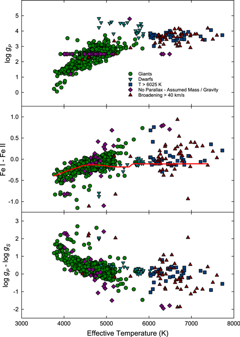
Figure 1. Top Panel—the mass-determined gravities vs. photometric temperature. The gravities, with a few exceptions, are as expected for giants. Middle Panel—the difference in the total iron abundance as determined from Fe i and Fe ii vs. effective temperature. The solid red line is a LOWESS smoothing of the differences for stars with [Fe/H] < −0.3. See Section 3.4.1 for a discussion. Bottom Panel—the difference in the mass-derived and ionization-balance gravities as a function of temperature. The implication is that if one accepts the validity of the ionization balance, there is a disconnect between atmospheric model structure and mass estimates derived from isochrones.
Download figure:
Standard image High-resolution imageThe next analysis parameter needed is the microturbulent velocity, which is found by demanding that the iron abundance as determined from Fe i lines show no dependence on equivalent width. Initial examination of Fe i data is often accompanied by an editing of the abundance data through an interactive line-editing process. However, in this case individual examination of each star is too time consuming. For Fe i, we assume there is no dependence of abundance on the excitation potential, and determine the best-fitting microturbulent velocity. The individual Fe i line abundances are then binned, and a Gaussian is fit to the Fe i histogram. Using a fit to the histogram deemphasizes the outliers and thus gives a better representation of the actual mean and dispersion. A symmetric 2σ clip is performed and the process repeated, except that in the second iteration a 2.5σ clip is done so that only real outliers will be eliminated. All stars are treated in this way, and the final clip line list is generated by tallying which lines are eliminated most often. The criterion for line elimination is that if a line is cut in 20% or more of the stars, it is eliminated in all stars by the final clip process. The number of Fe i lines prior to clipping is of order 700; after clipping it is about 500. Fe ii has an insufficient numbers of lines to pursue such a statistical process. Thus, for Fe ii, if there are more than 50 lines then the highest 10 and the lowest 3 are eliminated; at more than 20 lines the cuts are seven high and two low. After the Fe ii cuts are accumulated, the overall cut list is assembled in the same fashion as for Fe i. The number of Fe ii lines is typically 40–60 before trimming and 30–50 afterward. After arriving at the final Fe i and Fe ii data for each star, the microturbulent velocity was tweaked to a final value.
The Fe i data provide excitation information that can be interpreted in terms of the effective temperature. After final line trimming and setting of the microturbulent velocity, the Fe i line data shows a mean  (
( = 5040/T and
  is the slope of the abundance versus excitation potential relation) of about −0.01, with an uncertainty of about the same value. At 4800 K, this translates into an increased effective temperature of about 50 K to achieve excitation balance. If one limits the effective temperature range to 4000–5500 K—the regime where the excitation analysis has highest sensitivity and accuracy—the mean temperature increase needed falls to about 25 K. These changes are well within the uncertainties of the changes, as well as the accuracy of the photometric effective temperatures; thus, to within the uncertainties, the excitation data is consistent with the photometric effective temperatures. A caveat here is that the editing of the Fe I lines assumes that there are no intrinsic temperature trends within the data. Inspection of the deleted Fe i lines finds no preference for them to be of any particular excitation energy or equivalent width.
In examining the Fe i and Fe ii data, an imbalance in the total iron abundance is found in the general sense that the mass-derived gravity is too high (i.e., the Fe ii derived total iron abundance exceeds the Fe i value; see Figure 1—middle panel). To rectify this a new gravity was determined using an ionization balance, which involves forcing the neutral and ionized species of iron to give the same total abundance using the gravity as the free parameter. This was done by interpolating a small grid of models and then determining the best-fit gravity and microturbulence together. Parameter confirmation was done by interpolating a new model at the proper parameters. The iron data relations were recomputed to confirm the ionization balance, along with the lack of dependence of iron abundance on line strength.
These stars exhibit a range of metallicities and this is taken into account as the analysis proceeds. Below [Fe/H] of −0.3, models with [M/H = −0.5 are used, from [Fe/H] of −0.3 to +0.15 solar metallicity models are employed, and above [Fe/H] = +0.15 models with [M/H] = +0.25 are used. The preferred models are 2 M⊙, α enhancement proportional to [Fe/H], moderate CN processing (i.e., carbon diluted to [C/Fe] = −0.13, nitrogen enhanced to [N/Fe] = +0.31 with 12C/13C = 20), and 2 km s−1 Doppler velocity. There is little effect on the abundances due to a change from 2 to 1 M⊙, or from a change of 2–5 km s−1, so if a preferred model is not available, a change in grid is made.
Table 3 includes parameters, iron abundance details, an average macroturbulent/rotational velocity, and lithium, carbon, and oxygen data. Information for both mass and ionization-balance derived gravities is presented. There are a few stars that lack parallax and/or photometric data. For these stars, identifiable in Table 3 by the lack of a mass-derived analysis, a traditional excitation and ionization-balance analysis was performed. Average abundances for 25 elements with Z > 10 are in Table 4. The averages have been computed in the same manner as for Fe ii, except no master kill list was generated for species other than iron. If the neutral and first ionized species are both available for an element, the final average is merely the average of all retained lines. Note that the Mn, Co, and Cu abundances have been computed allowing for hyperfine structure. Details of the abundances (per species average, σ, and number of lines) are available upon request.
Table 3. Stellar Parameters, Fe, C, O, Li Abundance Data
| KeyName | Group 1a | Group 2b | |||||||||||||||||||||||||||||
|---|---|---|---|---|---|---|---|---|---|---|---|---|---|---|---|---|---|---|---|---|---|---|---|---|---|---|---|---|---|---|---|
| S | T | g | Vt | Fe i | S | N | Fe ii | S | N | C | O | Li | EW | N1 | T | G | Vt | Fe i | S | N | Fe ii | S | N | C | O | Li | N2 | Vm | B | Cl | |
| hd001671 | E | 6323 | 3.61 | 2.61 | 0.02 | 0.22 | 85 | 0.26 | 0.14 | 7 | 7.95 | 8.93 | 2.77 | 5.24 | 0.02 | 6323 | 2.95 | 2.71 | 0.00 | 0.22 | 85 | 0.01 | 0.15 | 7 | 7.75 | 8.74 | 2.77 | 0.05 | 44.0 | R | 2 |
| hd002910 | E | 4696 | 2.60 | 1.36 | 0.15 | 0.14 | 534 | 0.35 | 0.21 | 50 | 8.39 | 8.82 | 0.45 | 1.28 | 0.23 | 4696 | 2.10 | 1.50 | 0.05 | 0.14 | 534 | 0.05 | 0.23 | 50 | 8.23 | 8.59 | 0.46 | 0.28 | 5.1 | G | 1 |
| hd004188 | E | 4793 | 2.49 | 1.39 | 0.07 | 0.12 | 549 | 0.19 | 0.19 | 54 | 8.15 | 8.74 | 0.31 | 0.68 | 0.21 | 4793 | 2.20 | 1.46 | 0.02 | 0.12 | 549 | 0.03 | 0.20 | 54 | 8.07 | 8.60 | 0.31 | 0.23 | 5.0 | G | 1 |
| hd004502 | E | 4570 | 2.25 | 2.88 | −0.31 | 0.41 | 52 | 1.14 | 1.24 | 6 | ⋯ | ⋯ | 1.05 | 6.75 | 0.29 | 4570 | 0.10 | 2.61 | −0.53 | 0.46 | 52 | 0.09 | 1.36 | 6 | ⋯ | ⋯ | 0.96 | 0.47 | 40.0 | R | 2 |
| hd005234 | E | 4422 | 1.87 | 1.58 | 0.02 | 0.17 | 506 | 0.14 | 0.21 | 41 | 8.10 | 8.67 | 0.38 | 2.75 | 0.34 | 4422 | 1.58 | 1.62 | −0.04 | 0.18 | 506 | −0.04 | 0.22 | 41 | 8.02 | 8.54 | 0.37 | 0.37 | 5.7 | G | 1 |
| hd006319 | E | 4755 | 2.74 | 1.38 | 0.24 | 0.14 | 531 | 0.36 | 0.18 | 45 | 8.48 | 9.00 | 0.24 | 0.67 | 0.20 | 4755 | 2.44 | 1.48 | 0.17 | 0.14 | 531 | 0.17 | 0.19 | 45 | 8.39 | 8.86 | 0.25 | 0.22 | 5.0 | G | 1 |
| hd010380 | E | 4154 | 1.50 | 1.83 | −0.11 | 0.19 | 470 | 0.14 | 0.23 | 36 | 8.18 | 8.71 | −0.49 | 1.08 | 0.38 | 4154 | 0.90 | 1.86 | −0.30 | 0.20 | 470 | −0.30 | 0.26 | 36 | 7.86 | 8.33 | −0.53 | 0.47 | 5.4 | G | 1 |
| hd011559 | E | 4947 | 2.80 | 1.33 | 0.17 | 0.11 | 550 | 0.33 | 0.20 | 58 | 8.24 | 8.83 | 0.42 | 0.55 | 0.16 | 4947 | 2.54 | 1.37 | 0.12 | 0.12 | 550 | 0.12 | 0.21 | 58 | 8.06 | 8.61 | 0.42 | 0.17 | 5.5 | G | 1 |
| hd013174 | E | 6710 | 3.25 | 6.00 | 0.52 | 0.43 | 24 | −0.02 | 0.02 | 2 | 7.62 | 8.70 | 2.66 | 2.40 | 0.07 | 6710 | 3.49 | 7.75 | 0.47 | 0.39 | 24 | −0.01 | 0.12 | 2 | 7.66 | 8.74 | 2.66 | 0.05 | 80.0 | R | 2 |
| hd013480 | E | 5082 | 2.68 | 2.89 | −0.02 | 0.37 | 104 | 0.39 | 0.67 | 10 | 8.24 | 9.25 | 1.82 | 7.61 | 0.14 | 5082 | 1.72 | 2.92 | −0.06 | 0.37 | 104 | −0.06 | 0.67 | 10 | 8.01 | 8.80 | 1.83 | 0.19 | 36.0 | R | 1 |
Notes. KeyName: Identifier, S: Source of Spectra.
aData for the mass-determined gravity: T: Effective temperature (Kelvins), G: Logarithm of the surface gravity (cm s−2), Vt: Mictoturbulent Velocity (km s−1), Fe i: [Fe/H] determined from Fe i–logarithmic with respect to the solar value = 7.47, S: Standard Deviation of Fe i derived [Fe/H] ratio, N: Number of Fe i lines used, Fe ii: [Fe/H] determined from Fe ii–logarithmic with respect to the solar value = 7.47, S: Standard Deviation of Fe ii derived [Fe/H] ratio, N: Number of Fe ii lines used, C: Carbon abundance with respect to log  H = 12, O: Oxygen abundance with respect to log H = 12, Li: Lithium abundance with respect to log H = 12, EW: Equivalent width in picometers of the lithium 670.7 nm feature. EW < 1.00 pm corresponds to an upper limit, N1: Lithium non-LTE abundance correction from the data of Lind et al. (2009).
bData for the ionization-balance determined gravity: T: Effective temperature (Kelvins), G: Logarithm of the surface gravity (cm s−2), Vt: Mictoturbulent Velocity (km s−1), Fe i: [Fe/H] determined from Fe i—logarithmic with respect to the solar value = 7.47, S: Standard Deviation of Fe i derived [Fe/H] ratio, N: Number of Fe i lines used, Fe ii: [Fe/H] determined from Fe ii–logarithmic with respect to the solar value = 7.47, S: Standard Deviation of Fe ii derived [Fe/H] ratio, N: Number of Fe ii lines used, C: Carbon abundance with respect to log H = 12, O: Oxygen abundance with respect to log H = 12, Li: Lithium abundance with respect to log H = 12, EW: Equivalent width of the lithium 670.7 nm feature, N2: Lithium non-LTE abundance correction from the data of Lind et al. (2009), Vm: Broadening velocity (km s−1), B: Type of broadening: G = Gaussian Macroturbulence R = Rotational, C1: Clump Star: 1 = True 2 = False.
H = 12, O: Oxygen abundance with respect to log H = 12, Li: Lithium abundance with respect to log H = 12, EW: Equivalent width in picometers of the lithium 670.7 nm feature. EW < 1.00 pm corresponds to an upper limit, N1: Lithium non-LTE abundance correction from the data of Lind et al. (2009).
bData for the ionization-balance determined gravity: T: Effective temperature (Kelvins), G: Logarithm of the surface gravity (cm s−2), Vt: Mictoturbulent Velocity (km s−1), Fe i: [Fe/H] determined from Fe i—logarithmic with respect to the solar value = 7.47, S: Standard Deviation of Fe i derived [Fe/H] ratio, N: Number of Fe i lines used, Fe ii: [Fe/H] determined from Fe ii–logarithmic with respect to the solar value = 7.47, S: Standard Deviation of Fe ii derived [Fe/H] ratio, N: Number of Fe ii lines used, C: Carbon abundance with respect to log H = 12, O: Oxygen abundance with respect to log H = 12, Li: Lithium abundance with respect to log H = 12, EW: Equivalent width of the lithium 670.7 nm feature, N2: Lithium non-LTE abundance correction from the data of Lind et al. (2009), Vm: Broadening velocity (km s−1), B: Type of broadening: G = Gaussian Macroturbulence R = Rotational, C1: Clump Star: 1 = True 2 = False.
Only a portion of this table is shown here to demonstrate its form and content. Machine-readable and Virtual Observatory (VOT) versions of the full table are available.
Download table as: Machine-readable (MRT)Virtual Observatory (VOT)Typeset image
Table 4. Average Element Abundances [x/H]
| Keyname | S | T | G | Vt | Na | Mg | Al | Si | S | Ca | Sc | Ti | V | Cr | Mn | Fe | Co | Ni | Cu | Zn | Sr | Y | Zr | Ba | La | Ce | Nd | Sm | Eu |
|---|---|---|---|---|---|---|---|---|---|---|---|---|---|---|---|---|---|---|---|---|---|---|---|---|---|---|---|---|---|
| Mass Determined Gravity Data | |||||||||||||||||||||||||||||
| hd001671 | E | 6323 | 3.61 | 2.61 | 0.11 | ⋯ | ⋯ | 0.17 | 0.55 | 0.22 | 0.33 | 0.33 | 0.82 | 0.44 | 0.06 | 0.03 | 0.39 | 0.33 | −0.59 | −0.35 | 1.46 | 0.91 | 1.97 | ⋯ | 0.25 | 0.29 | 0.41 | 0.78 | |
| hd002910 | E | 4696 | 2.60 | 1.36 | 0.30 | 0.26 | 0.22 | 0.41 | 1.02 | 0.17 | 0.13 | 0.12 | 0.27 | 0.22 | 0.19 | 0.17 | 0.11 | 0.26 | 0.30 | 0.71 | 0.02 | 0.22 | −0.02 | 0.12 | 0.56 | 0.86 | 0.50 | 0.43 | 0.21 |
| hd004188 | E | 4793 | 2.49 | 1.39 | 0.29 | 0.22 | 0.26 | 0.25 | 0.70 | 0.11 | 0.03 | 0.08 | 0.17 | 0.16 | 0.11 | 0.08 | 0.03 | 0.12 | 0.12 | 0.35 | 0.12 | 0.20 | 0.04 | 0.12 | 0.44 | 0.65 | 0.38 | 0.40 | 0.14 |
| hd004502 | E | 4570 | 2.25 | 2.88 | ⋯ | ⋯ | 0.08 | 0.69 | ⋯ | −0.07 | 0.06 | 0.00 | −0.04 | −0.01 | −0.16 | −0.16 | 0.15 | −0.02 | ⋯ | ⋯ | ⋯ | −0.03 | 0.82 | ⋯ | 0.85 | ⋯ | 0.48 | 0.84 | 0.44 |
| hd005234 | E | 4422 | 1.87 | 1.58 | 0.27 | 0.09 | 0.21 | 0.41 | 0.81 | −0.01 | −0.08 | 0.02 | 0.06 | 0.18 | 0.04 | 0.03 | −0.06 | 0.08 | 0.12 | −0.29 | 0.06 | 0.04 | −0.11 | 0.13 | 0.50 | 0.81 | 0.52 | 0.79 | 0.06 |
| hd006319 | E | 4755 | 2.74 | 1.38 | 0.38 | 0.29 | 0.42 | 0.37 | 0.95 | 0.18 | 0.30 | 0.32 | 0.48 | 0.31 | 0.30 | 0.25 | 0.25 | 0.35 | 0.48 | 0.46 | 0.17 | 0.26 | 0.17 | 0.28 | 0.68 | 0.90 | 0.75 | 0.67 | 0.31 |
| hd010380 | E | 4154 | 1.50 | 1.83 | 0.19 | 0.26 | 0.13 | 0.33 | 1.16 | −0.20 | −0.13 | −0.09 | −0.02 | 0.01 | −0.14 | −0.09 | 0.01 | 0.03 | 0.18 | 0.23 | −0.06 | −0.11 | −0.25 | −0.23 | 0.31 | 0.30 | 0.37 | 0.33 | −0.03 |
| hd011559 | E | 4947 | 2.80 | 1.33 | 0.46 | 0.27 | 0.31 | 0.37 | 0.86 | 0.21 | 0.12 | 0.18 | 0.27 | 0.27 | 0.18 | 0.19 | 0.14 | 0.22 | 0.23 | 0.22 | 0.19 | 0.29 | 0.09 | 0.23 | 0.45 | 0.75 | 0.53 | 0.47 | 0.35 |
| hd013174 | E | 6710 | 3.25 | 6.00 | −1.12 | ⋯ | ⋯ | 0.30 | ⋯ | 1.30 | 0.75 | 1.34 | 1.36 | 0.37 | −0.09 | 0.48 | 1.58 | 0.42 | ⋯ | ⋯ | 0.55 | −0.11 | 2.23 | ⋯ | ⋯ | 0.11 | 0.72 | 1.32 | 0.72 |
| hd013480 | E | 5082 | 2.68 | 2.89 | ⋯ | ⋯ | ⋯ | 0.18 | 0.47 | 0.08 | 0.02 | 0.28 | 0.37 | 0.59 | −0.26 | 0.01 | 0.39 | 0.09 | −0.55 | ⋯ | 2.30 | 0.23 | 1.29 | −0.15 | 0.65 | 0.66 | 0.98 | 0.56 | 0.89 |
Notes. Keyname: Identifier, S: Source of Spectra, T: Effective temperature (Kelvins), G: Logarithm of the surface gravity (cm s−2), Vt: Mictoturbulent Velocity (km s−1), Na: Logarithmic sodium abundance with respect to the solar value, Mg: Logarithmic magnesium abundance with respect to the solar value, Al: Logarithmic aluminum abundance with respect to the solar value, Si: Logarithmic silicon abundance with respect to the solar value, S: Logarithmic sulfur abundance with respect to the solar value, Ca: Logarithmic calcium abundance with respect to the solar value, Sc: Logarithmic scandium abundance with respect to the solar value, Ti: Logarithmic titanium abundance with respect to the solar value, V: Logarithmic vanadium abundance with respect to the solar value, Cr: Logarithmic chromium abundance with respect to the solar value, Mn: Logarithmic manganese abundance with respect to the solar value, Fe: Logarithmic iron abundance with respect to the solar value, Co: Logarithmic cobalt abundance with respect to the solar value, Ni: Logarithmic nickel abundance with respect to the solar value, Cu: Logarithmic copper abundance with respect to the solar value, Zn: Logarithmic zinc abundance with respect to the solar value, Sr: Logarithmic strontium abundance with respect to the solar value, Y: Logarithmic yttrium abundance with respect to the solar value, Zr: Logarithmic zirconium abundance with respect to the solar value, Ba: Logarithmic barium abundance with respect to the solar value, La: Logarithmic lanthanum abundance with respect to the solar value, Ce: Logarithmic cerium abundance with respect to the solar value, Nd: Logarithmic neodymium abundance with respect to the solar value, Sm: Logarithmic samarium abundance with respect to the solar value, Eu: Logarithmic europium abundance with respect to the solar value.
Only a portion of this table is shown here to demonstrate its form and content. Machine-readable and Virtual Observatory (VOT) versions of the full table are available.
Download table as: Machine-readable (MRT)Virtual Observatory (VOT)Typeset image
3.3. Li, C, N, and O Analysis
For lithium, carbon, nitrogen, and oxygen, spectrum syntheses for the features of interest have been performed using laboratory oscillator strengths where available. For the lithium feature, all components of 7Li (using the data presented by Andersen et al. 1984) in the 670.7 nm hyperfine doublet were used to match the observed profiles. There is no evidence in the observed spectra for the presence of 6Li, and therefore it was not considered in the syntheses. Lithium LTE abundance data are presented in Table 3, including the synthesized equivalent width of the Li blend. Also included are non-LTE lithium abundance corrections from the data of Lind et al. (2009).
Carbon abundances have been derived from C i lines at 505.2 nm and 538.0 nm, and the C2 Swan system lines at 513.5 nm. For the atomic lines, the oscillator strengths of Biémont et al. (1993) or Hibbert et al. (1993) were adopted. These oscillator strengths have been used in determinations of the solar carbon abundance (Asplund et al. 2005). For the Swan C2 syntheses, f (0, 0) = 0.0303 (Grevesse et al. 1991) was adopted with the relative band f values of Danylewych & Nicholls (1974), along with D0 = 6.210 eV (Grevesse et al. 1991) and theoretical line wavelengths (as needed) from C. Amiot (1982, private communication). To form the carbon abundance on a per spectrum basis, the individual features are combined as follows: for Teff < 4800 K: C2 513.5 only. At T > 4800 K and less than 5500 K, C i 505.2 and 538.0 have weight 1 and C2 513.5 has weight 3. For T > 5500 K, the two C i lines have equal weight and C2 is not used. The weights are based on relative strength and blending. Typical spreads in abundance for the features are 0.15 dex. For the purpose of abundances with respect to solar values, we adopt log C = 8.43, which is the Asplund et al. (2009) recommended solar carbon abundance. Table 3 has the average C and O data on a per star basis.
Oxygen abundance indicators in the available spectral range are rather limited: the O i triplet at 615.6 nm and the [O i] lines at 630.0 and 636.3 nm. The O i 615.6 nm lines are problematic in abundance analyses with only the 615.8 nm line being retained in solar oxygen analyses (Asplund et al. 2004). The O i lines were synthesized using the NIST atomic parameters (Kramida et al. 2013) that were also used by Asplund et al. (2009). For the forbidden oxygen lines, only 630.0 nm is usable because 636.3 nm is weak, heavily blended, and complicated by the presence of the Ca i autoionization feature. In the syntheses of 630.0 nm, the line data presented by Allende Prieto et al. (2001) was used, except that the experimental oscillator strength for the blending Ni i line (Johansson et al. 2003) was adopted. The syntheses assumed [Ni/Fe] = 0. In G and K giants, the [O i] 630.0 nm equivalent width typically runs from 3 to 8 nm, and the Ni i intrusion about 0.5 nm. An uncertainty of 20% in the Ni I strength is therefore not a major concern. To form a final oxygen abundance, the data was average in the following manner: for Teff < 5500 K,only [O i] is used, whereas for Teff > 5500 K, O i has weight 1 and [O i] has weight 3. At an effective temperature of 6225 K, [O i] is essentially undetectable and the abundance depends only on O i 615.8 nm. For Teff < 5500 K, the C–O dependence has been explicitly taken into account.
3.4. Abundance and Parameter Comparisons
3.4.1. Internal Comparison
This study affords two types of internal comparisons: there are 19 stars with two analyses, and for each star/spectra there is the mass-derived gravity abundance determination and the ionization-balance gravity analysis. The 19 stars with two analyses shall be dealt with first.
Comparing the effective temperature data for the 19 stars, a mean difference of 4 K with a total range of 39 to −20 K is found. There can be a difference because the determinations were made for each data source separately, without reference any previous determination, and thus different colors can be eliminated in each determination. Note that a difference of 40 K in this temperature range is less than 1% in the temperature. The mass-derived gravities show a mean difference of 0 with a total range of −0.08 to +0.05 dex. The abundance data associated with the mass-derived gravity is very consistent: the mean differences for iron (Fe i), carbon, and oxygen are −0.01, −0.01, and −0.02, respectively. The standard deviation about the mean is of order 0.1 for three species. For the ionization-balance gravities, the mean difference in log g is 0.08 dex (σ = 0.12). The mean difference for the iron, carbon, and oxygen abundance between the two analyses is about 0.02 dex for each species, with the standard deviation once again being of order 0.1 dex.
As noted, the total data set shows a systematic difference in the gravities derived from the mass and from the ionization balance. The iron abundance difference (Fe i−Fe ii) in the mass-derived gravity analysis is dependent on the temperature: at 5000 K the difference is of order 0.2 dex increasing to about 0.5 dex at 4000 K—see Figure 1 (middle panel). In comparing the mass-derived and ionization-balance gravities, this difference manifests itself as progressively larger differences between the two as a function of effective temperature (bottom panel of Figure 1). Bruntt et al. (2011) noted this type of variation in Kepler field red giants using astroseismology-determined parameters. The effect is also present in the data of LH07. The dependence of the gravity difference on the effective temperature could indicate a failure in the model atmospheres. However, a brief sanity check using ATLAS9 models (Kurucz 1992) yields the same results to within 0.1 dex in log g and 0.05 dex in total iron abundance. The mass difference implied by the change in gravity is certainly non-physical. A 0.2 dex lower gravity at constant temperature and luminosity yields a 40% lower mass, whereas lowering the gravity by 0.6 dex implies a 75% lower mass. The average mass then would decrease to 0.5–1.0 solar masses depending on the temperature, which is not an especially appealing result.
Smoothed (x I–x II) data is presented for Ti, V, Cr, and Fe in Figure 2 (top panel). The immediate conclusion drawn from this figure is that all of these species suffer from the same problem. Whatever is affecting iron also affects the ionized data of other species, and yields the same problem relative to the neutral species: the total abundance inferred from the first ionized species is too large. The ionization balance performed using Fe i and Fe ii rectifies most of the problems, with the difference between the Ti, V, and Cr neutral and ionized total abundances declining; but, more important, the dependence on effective temperature is ameliorated (see bottom panel of Figure 2).
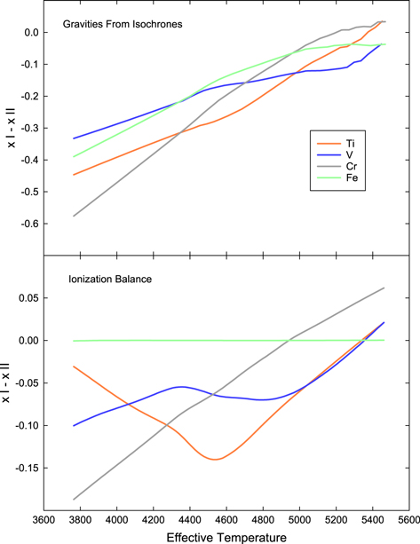
Figure 2. LOWESS smoothed differences in Ti i–Ti ii, V i–V ii, Cr i–Cr ii, and Fe i–Fe ii as a function of effective temperature. Outliers have been eliminated in each smoothing. The top panel shows the difference for the mass-derived gravities and the bottom for the ionization-balance gravities. The mass-derived gravity differences for Ti, V, and Cr are similar in form to the differences for Fe, indicating that a common failure is leading to the difference.
Download figure:
Standard image High-resolution imageA possible reason behind this problem is that the ionized lines, and specifically the Fe ii lines, are affected by progressively stronger blending with decreasing temperature. While possible, this would demand that that all Fe ii lines be similarity affected. A weak check is available on this possibility: metal-poor giants should not show the effects of line blending to the extent that solar or above-solar abundance giants do. This is not true if the features in the Fe ii blend are nearly coincident in wavelength. The situation envisioned here is that lines within 0.015 nm of an Fe ii line progressively make the centroid and FWHM of the Fe ii line less secure, as the overall line strength increases with decreasing temperature. Since metal-poor stars have intrinsically weaker lines, their lines should remain less "blended." In the middle panel of Figure 1, the solid red line is the smoothed differences in Fe i–Fe ii computed from stars with [Fe/H] < −0.3. In the smoothing, outliers have been excluded although they tend to exhibit large overabundances of Fe ii. As can be seen, the metal-poor-stars show differences that indicate that Fe ii is larger than Fe i in the bulk of sample, and in the 4500 K and below region the differences tail off in much the same way as the entire sample. While not conclusive, this indicates that line blending in Fe ii is not the sole culprit of the problem.
Two other possibilities relative to the gravity are significant non-LTE effects in iron, or that lower temperature, lower gravity stellar atmospheric models do not reflect the actual structure of stars. The latter possibility is difficult to assess, but the non-LTE alternative has been examined in other studies.
The first study of non-LTE effects in iron in cooler stars is likely that of Tanaka (1971), and these studies have proceeded through the work of Mashonkina et al. (2011) to the review by Mashonkina (2013), as well as the studies of Ezzedine et al. (2013) and Lapenna et al. (2014). The primary results from the latter two papers are that non-LTE calculations may yield better agreement between Fe i and Fe ii using parameters much like the mass-derived parameters used here, and that the non-LTE effects become stronger with decreasing temperature and metallicity. The non-LTE abundances found are closer to the LTE Fe ii values, but depend strongly on the poorly known strength of inelastic hydrogen collisions.
A counterpoint to the discussion above is found in arguments presented by Morel et al. (2014) and Adamczak & Lambert (2014). Both works argue that a traditional excitation and ionization analysis to determine stellar parameters is a valid approach. They cite the work of Bergemann et al. (2012) and Lind et al. (2012) as showing that iron is not significantly affected by departures from LTE, especially at higher abundances, such as those found in their study and by extension, those determined here. A quandary thus exists at this point as to the importance of non-LTE effects in iron, the resolution of which lies beyond the scope of this work; the priority in this analysis will be to maximize the reliability of these abundances under the current analysis constraints.
At temperatures above 5500 K there is a large spread in in the mass-derived and ionization-balance gravities (see Figure 1, bottom panel). This is because the ionization balance is susceptible to large uncertainties in Fe i and Fe ii equivalent widths. The equivalent width uncertainty arises due to the large (>20 km s−1) line broadening seen in these stars.
3.4.2. External Comparison
To locate previous analyses of the program stars, the PASTEL database (Soubrian et al. 2010) was consulted. More than 720 of the program stars have data in PASTEL. The total number of references generated was in excess of 215, which does not include a number of analyses published post 2012. We selected a subset of the available data to investigate the parameter and abundance comparison.
For the first comparison, the obvious choice is LH07, which has corresponding data on 288 stars. LH07 also used photometric temperatures, but with a different calibration, and mass-derived gravities as part of their analysis. The mean differences relative to this study are small: −42 K in temperature (σ = 78 K), +0.02 in mass-derived log g (σ = 0.14), and +0.10 in [Fe i/H] (σ = 0.07). The sense is this study minus LH07. This study uses a different line list with newly determined solar oscillator strengths. Part of the difference in the iron abundance arises from the selected solar reference point, but quantification is difficult because LH07 zero pointed each line abundance individually, whereas here a single solar abundance is used and the gf value adjusted to match the solar line strength.
Hekker & Meléndez (2007) performed a traditional spectroscopic parameter determination (i.e., an excitation and ionization balance) on 189 of the stars considered here. The mean offsets in effective temperature, gravity, and [Fe/H] are −96 K (σ = 78), −0.35 dex (σ = 0.25), and +0.03 dex (σ = 0.11), respectively, for the mass-determined gravity and Fe i abundance. The differences for the ionization-balance analyses are −0.58 dex (σ = 0.76) in log g, and −0.01 dex (σ = 0.09) for Fe i. The differences are in the sense this work minus Hekker & Meléndez. The number of lines used by Hekker & Meléndez was 20 Fe i lines and 6 Fe ii lines versus 400 Fe i lines and 33 Fe ii lines used on average here. A comparison of the gf values between the two studies shows good agreement: a mean difference in log gf of −0.05 for Fe i and a difference of −0.02 for Fe ii, in the sense Hekker & Meléndez minus the work. There is considerable scatter in the gravities, but this is expected given the small number of Fe ii lines used in Hekker & Meléndez. The systematic offset in gravity cannot be explained by the difference in temperature. In an ionization balance, an effective temperature increase would demand an increase in the gravity, but a 100 K difference does not explain the 0.6 dex shift seen here in the ionization-balance gravities. Additionally, the systematic gravity difference is unlikely to be explained by postulating that the masses found here are underestimated. To rectify the mass gravities found here with the Hekker & Meléndez values, an increase of a factor of two in mass would be required, yielding a mean mass of about 3.5 solar masses. Note that the mass derivation is relatively insensitive to the temperature; numerical experiment shows that the mass increases by about 0.1 solar mass for a temperature change of +100 K. Given the differences in effective temperature and gravity between these two works, the small difference in mean iron abundance is remarkable.
Takeda et al. (2008) analyzed a sample of 322 K giants, of which 191 are in common with this work. Their analysis uses an excitation and ionization-balance technique to derive parameters. The mean difference in effective temperature (this work—Takeda et al.) is −51 K, with a standard deviation of 68 K. The individual temperature differences can be significant: the total spread is −430 to +245 K. Comparing the log g values, the mean difference is −0.12 (σ = 0.10) using the mass gravities given here. For the ionization-balance gravities of this work, the difference is −0.31 (σ = 0.19). Once again, the remarkable thing is the agreement of the iron abundances: the mean difference is +0.05 dex (σ = 0.06) for the mass gravity iron abundance derived from Fe i, whereas the mean difference in iron is +0.02 dex for the ionization-balance gravities.
Liu et al. (2014) analyzed lithium in a sample of 378 giants, taking the parameters from Takeda et al. (2008) and Liu et al. (2010). The parameters of Takeda et al. relative to this study are discussed above and the parameters of Liu et al. (2010) give similar results. Comparison of the Liu et al. (2014) lithium abundances to those found here shows that the abundance differences correlate well with the temperature differences. This is expected based upon the sensitivity of the lithium abundance on the temperature. Where the temperatures agree to within 25 K, the lithium abundances agree to better than 0.1 dex. There is considerable scatter about the mean difference line, but this is also expected because the lithium feature is very weak in these stars: the median equivalent width in the 200+ stars in common is about 0.75 pm, with a maximum of 6.5 pm. Most of the abundances are considered to be limits only in this work.
Another traditional spectroscopic analysis is that of Da Silva et al. (2011), who analyzed 172 stars, of which 98 are included in this work. Comparing their excitation temperatures with the photometric temperatures of this work shows a mean difference of −93 K with a standard deviation of 125 K. The range is quite large: the differences span −283–900 K, in the sense of this work—Da Silva et al. The gravities differ by −0.22 (σ = 0.22) for the mass gravities determined here and by −0.46 (σ = 0.31) for the ionization-balance values. As seems to be the usual case, the iron abundances are in rather good agreement in the mean: +0.06 (σ = 0.11) for the mass determination and +0.01 (σ = 0.11) for the ionization-balance gravities.
Recent advances in observational techniques, specifically, the photometric capabilities of the Corot and Kepler satellites, have allowed seismic techniques to be applied to stars. This development permits the determination of gravities with high precision. The studies using seismic techniques generally consider samples of 20–40 stars, and there is not a large overlap with this work. However, the power of astroseismology warrants some discussion relative to the results determined here. Three studies of particular interest are Morel & Miglio (2012), Creevey et al. (2013), and Morel et al. (2014). There are 12 stars in common with this work, of which six appear in two of the cited papers. The first observation is that the temperatures used in the astroseismology work are usually within 100 K of the temperature derived here. Comparing the seismic gravities to the isochrone values, the difference is of order −0.05 (with this work being the lower); whereas the spectroscopic gravity values determined here are of order −0.4 dex lower, as expected. This means that the differences in this work's parameters noted relative to other techniques and studies are comparable to those found, relative to determinations using seismic data.
In the past several years a number of other studies (e.g., Wang et al. 2011; Mortier et al. 2013; Ramírez et al. 2013) have considered 5–20 of the giants analyzed here. Comparison of the results show no surprises, the differences in temperature and gravity are consistent with those noted above; per usual, the [Fe/H] values are in good agreement.
Another compendium of parameters that warrants mention, perhaps more as a caveat emptor, is that of McDonald et al. (2012). Effective temperatures and luminosities are derived therein for the bulk of the Hipparcos stars by fitting spectral energy distributions to a variety of photometry. More than 900 of the stars considered in this work are found in McDonald et al. The mean temperature difference is −113 K (this work—theirs), with a standard deviation of 133 K. The luminosities agree rather well—the mean difference is +0.02 in log L/L⊙. While the mean offsets are not especially troubling, the range of temperature differences relative to this study, ±600 K, is rather distressing. This range is found after eliminating their temperature of 17296 K for ν Hya (K0/K1 III) and 10700 K for μ Vir (F2 V). There are two immediately apparent problems in McDonald et al. First, they do not include any reddening, and second, their classification method makes most of the giants analyzed here dwarfs. While the results are sufficiently accurate for their purpose, the temperatures are unsuited for use in an analysis such as this one.
4. DISCUSSION
4.1. Sample Culling
Figure 3 shows an HR diagram of the program stars along with mass tracks from Bressan et al. (1993). The tracks are only to serve as an indicator of mass and evolutionary status. The stars shown in this plot form the first cut on the sample: only stars with a Hipparcos parallax or in a cluster are retained. The stars are also identified by broadening velocity (Vm), which can be either a macroturbulent or rotational velocity (see Table 3). The stars with Vm > 40 km s−1 are mostly rotating F giants coming off the Main Sequence. In fact, most of the stars blueward of log Teff > 3.78 are fast rotators, leading to difficulties in determining accurate line strengths due to velocity smearing of the profiles. As a result, stars with effective temperatures in excess of 6025 K are eliminated from further discussion.

Figure 3. HR diagram for the program stars. The stars to the right of the vertical line at log (Teff) = 3.78 and above the diagonal line form the "clump" sample and are indicated by a "1" in last column of Table 3; the remainder are designated by a "2."
Download figure:
Standard image High-resolution imageA number of potential dwarfs are seen in Figure 1 (top panel). These are the stars below the diagonal line starting at log Teff = 3.78 and log L/LSun = +1.4 in Figure 3, and going toward lower temperatures and luminosities, and are eliminated from further discussion. In addition, 12 more stars are removed due to the inability to reach a spectroscopic ionization equilibrium inside the model grids. After the culling, 1006 G and K giants remain. In Table 3 last column, the retained stars are denoted by a "1" and the excluded stars a "2."
4.2. Mass versus Ionization Balance Gravity
The next question to be addressed is which analysis—mass or ionization balance—is more reliable and hence, the basis for further discussion. Figure 4 presents a histogram of the ionization-balance [Fe/H] data, along with a Gaussian fit to the data, the Gaussian centroid values for the mass-derived Fe i and Fe ii data, and the simple mean value for the ionization-balance [Fe/H] values. The Gaussian fits to the distributions all have similar standard deviations of about 0.17 dex. The slight asymmetry in the [Fe/H] distribution is real, as there are more metal-poor than metal-rich stars in the local region. Note that three very metal-poor stars are cut off from the plot, but are included in the fit. The metal-poor asymmetry leads to the difference of 0.1 dex between the simple average and the centroid of the ionization-balance data.
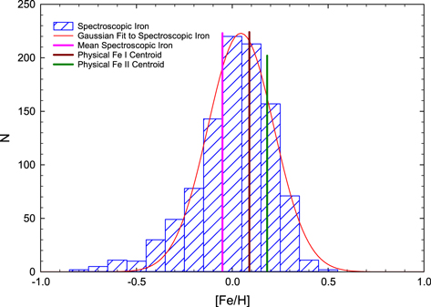
Figure 4. Histogram of iron abundances derived from the "clump" sample—see Section 4.1 for a formal definition. The Gaussian fit to the data yields a centroid abundance [Fe/H] = 0.089 that is about 0.04 larger than the simple mean. The centroid values for Fe i and Fe ii for the mass-derived gravity abundances are higher than the iron centroid for the ionization-derived gravities, with Fe ii deviating the most.
Download figure:
Standard image High-resolution imageThe metallicity of the local region as evidenced by F, G, and K dwarfs is close to solar (Luck & Heiter 2005, 2006). While the G and K giants of this study are not necessarily coeval with the dwarfs of the local region, one could expect the abundances for larger, non-biased samples for each to be commensurate. While the centroid values for the mass-derived gravity Fe i data and the ionization-balance [Fe/H] values are not vastly different—0.09 and 0.05 dex, respectively—and fall close to our expectation of solar abundance, the mass-derived Fe ii centroid value of +0.18 dex is uncomfortably high.
Another reason for favoring the ionization-balance gravity is that [x/Fe] ratios where x is a specified element are central to the discussion. Such ratios are used to help minimize parameter sensitivity. To form these ratios, one uses total abundances from species with like sensitivity to parameters; in general, ion to ion and neural to neutral. The advantage of the ionization gravities is that neutral and ionized total abundances are equivalent—at least in theory—in practice they are closer than those yielded by the mass gravity (see Figure 2), but are not perfectly matched. Use of the ionization-balance gravity thus allows the formation of the ratio without explicitly worrying about parameter sensitivity. Accordingly, the abundances for the primary discussion will be those of the ionization-balance analysis, with the mass values at the periphery. The mass gravity parameters and abundances are included in the tables, so an interested user can explore that data if so inclined.
4.3. Z > 10 Abundances
Hinkel et al. (2014) gave an extensive discussion of metallicity trends in the local region. While the stars considered in that work are dwarfs, the trends versus [Fe/H], velocity, and position discussed therein are not significantly different from those found in local giants. The history of nucleosynthesis for both local dwarfs and giants is very similar; thus only a brief discussion will be given here to point out salient features in the giant abundances.
Figure 5 presents the average [x/Fe] data for the G and K giants of this study. In this notation, "x" represents a target element. This distribution is much like that of LH07 (see their Table 10) for most elements. The most striking items in Figure 5 are the behaviors of sulfur and zinc. The zinc lines are badly blended, especially at temperatures below 4800 K, resulting in abundances of poor quality. The difficulty with sulfur is a ferocious temperature dependence in the data—see Figure 6. The span in the abundances is over two orders of magnitude, rising from [S/Fe] about +0.2 at 5240 K to greater than +2 at 4000 K. Once again, the problem is blends in the relevant lines. Hyperfine structure was not considered for Mn, Co, and Cu in the analysis of LH07; whereas the abundances here do account for hyperfine structure. However, the mean abundances in this analysis are not vastly different from those of LH07.
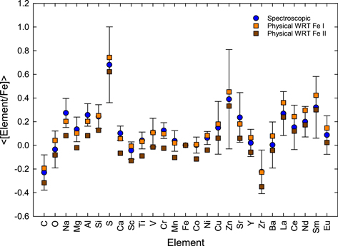
Figure 5. Average ionization-balance abundances with respect to iron as a function of element (Z). The two most deviant points are sulfur and zinc. The latter is based on a small number of unreliable lines. The cause for the sulfur "overabundance" is shown in Figure 6. The error bars are one standard deviation about the mean value.
Download figure:
Standard image High-resolution image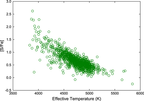
Figure 6. Sulfur abundances as a function of effective temperature. A clear-cut temperature effect is seen, which stems from the high potential sulfur lines being strongly blended with increasing contributions from other species as the temperature decreases.
Download figure:
Standard image High-resolution imageAnother way of looking at Z > 10 abundances is to examine either [x/H] or [x/Fe] as a function of [Fe/H]. The overall expectation is that in a sample of disk G and K giants, both [x/H] and [x/Fe] should track [Fe/H]; that is, the slope of [x/H] versus [Fe/H] should be about 1 and the intercept [x/H] should be close to the mean value in the local region. For [x/Fe], the slope should be about 0, with the intercept having the local region [x/Fe] value. There will obviously be exceptions and the strength of the deviations will depend on how metal-poor the stars are. In this sample, we look at the trends down to [Fe/H] = −0.8 and throw out only the four most metal-poor stars. Table 5 gives the values and uncertainties in the trends versus [Fe/H], along with mean values. The expectations are born out in large part in the data. The exceptions, unsurprisingly, are carbon, oxygen, and the α-elements. Other elements, Mn for example, also show gradients with respect to iron. Carbon and oxygen will be discussed in the following section. Note that the gradients in Table 5 do not allow for different slopes as a function of [Fe/H]. This data set is too heavily dominated by thin disk stars to discern differences due to the thin versus the thick disk.
Table 5. Gradients with respect to [Fe/H] for Ionization Balance Abundances
| [Element/H]=Slope*[Fe/H]+Int | [Element/Fe]=Slope*[Fe/H]+Int | ||||||||||||||
|---|---|---|---|---|---|---|---|---|---|---|---|---|---|---|---|
| Element | Slope | Int | e_Slope | e_Int | ∑ | Mean | σ | Slope | Int | e_Slope | e_Int | ∑ | Mean | σ | N |
| C | 0.617 | −0.249 | 0.020 | 0.004 | 0.126 | −0.278 | 0.177 | −0.382 | −0.249 | 0.020 | 0.004 | 0.126 | −0.231 | 0.148 | 964 |
| O | 0.574 | −0.056 | 0.021 | 0.004 | 0.128 | −0.084 | 0.173 | −0.426 | −0.056 | 0.021 | 0.004 | 0.128 | −0.036 | 0.154 | 963 |
| C/O | 0.040 | 0.364 | 0.014 | 0.003 | 0.090 | 0.363 | 0.090 | ⋯ | ⋯ | ⋯ | ⋯ | ⋯ | ⋯ | ⋯ | 963 |
| Na | 1.082 | 0.280 | 0.019 | 0.004 | 0.121 | 0.230 | 0.249 | 0.083 | 0.280 | 0.019 | 0.004 | 0.121 | 0.276 | 0.122 | 1002 |
| Mg | 0.782 | 0.124 | 0.014 | 0.003 | 0.092 | 0.088 | 0.182 | −0.218 | 0.125 | 0.014 | 0.003 | 0.092 | 0.135 | 0.102 | 997 |
| Al | 0.833 | 0.249 | 0.014 | 0.003 | 0.089 | 0.211 | 0.190 | −0.167 | 0.250 | 0.014 | 0.003 | 0.089 | 0.257 | 0.095 | 1000 |
| Si | 0.817 | 0.234 | 0.015 | 0.003 | 0.092 | 0.197 | 0.189 | −0.183 | 0.235 | 0.015 | 0.003 | 0.093 | 0.243 | 0.100 | 1004 |
| Ca | 0.886 | 0.096 | 0.009 | 0.002 | 0.054 | 0.055 | 0.187 | −0.114 | 0.096 | 0.009 | 0.002 | 0.055 | 0.101 | 0.059 | 1004 |
| Sc | 0.940 | −0.047 | 0.011 | 0.002 | 0.072 | −0.090 | 0.202 | −0.059 | −0.047 | 0.011 | 0.002 | 0.072 | −0.044 | 0.073 | 1004 |
| Ti | 0.926 | 0.037 | 0.011 | 0.002 | 0.068 | −0.006 | 0.199 | −0.073 | 0.037 | 0.011 | 0.002 | 0.069 | 0.040 | 0.070 | 1004 |
Notes. e_Slope = Standard error of the slope, e_Int = Standard error of the intercept, ∑ = Standard deviation of the fit, Mean = Mean of the ratios, σ = Standard deviation of the mean, N = Number of stars.
Only a portion of this table is shown here to demonstrate its form and content. Machine-readable and Virtual Observatory (VOT) versions of the full table are available.
Download table as: Machine-readable (MRT)Virtual Observatory (VOT)Typeset image
The behavior of the α-elements is well documented in the literature (see, e.g., McWilliam 1997; Allende Prieto et al. 2004; LH07; Hinkel et al. 2014). Shown in Figure 7 (top panel) is the behavior of [Si/Fe] versus [Fe/H]. As expected, [Si/Fe] increases with decreasing [Fe/H]. While the effect is modest, it is real and persists through Ca. Note that a loess smoothing of the data—the gradients in the figure—yields a result akin to the linear fit. The root cause for the decrease in [α/Fe] as [Fe/H] increases is the growing dominance of SN Ia production of the Fe-peak elements over the production of lighter α-elements in SN II as the galaxy ages.

Figure 7. [Si/Fe], [Mn/Fe], and [Co/Fe] as a function of [Fe/H]. Silicon and manganese show definite trends vs. [Fe/H], but [Co/Fe] does not. The solid black line is a linear fit to the data, while the red line is a LOESS smoothing. All three elements show a dip at about [Fe/H] = 0. The error bars are the mean standard deviation of each species taken across the sample. See text for discussion.
Download figure:
Standard image High-resolution image[Mn/Fe] versus [Fe/H] is shown in the middle panel of Figure 7. There is a definite slope in the data, with lower [Fe/H] ratios showing lower [Mn/Fe]. This effect was noted by LH07 and first demonstrated by Wallerstein (1962) and Wallerstein et al. (1963). Gratton (1989) also noted the effect in a sample of metal-poor to solar-metallicity stars. The effect is the reverse of the trends seen in the α-elements and presumably indicates an SN Ia origin for Mn. However, the adjoining odd elements V and Co show no believable trend with [Fe/H]—see the bottom panel of Figure 7 for Co.
The dwarf data from the Hypatia Catalog (Hinkel et al. 2014) show a curious phenomenon in the Ni abundances. Two [Ni/Fe] ratios appear in the data at essentially all [Fe/H] ratios. There is a group at a slightly subsolar ratio, [Ni/Fe] ∼ −0.03, and another at [Ni/Fe] ∼ −0.2. Hinkel et al. also delineate the abundances based on distance from the Sun. In Figure 8, [Ni/Fe] is presented as a function of [Fe/H], with the stars delineated by heliocentric distance. There is no discernible dependence in the data as a function of distance. There appears to be a downward trend in [Ni/Fe] with decreasing [Fe/H]. The data smoothing shows a flat dependence at [Fe/H] < 0, with increasing [Ni/Fe] for [Fe/H] > 0. There is also a dip in [Ni/Fe] at [Fe/H] about [Fe/H] = 0. However, the actual spread in the data is small. In the bin −0.2 < [Fe/H] < +0.2, the mean [Ni/Fe] ratio is +0.058 with a standard deviation of 0.053 (N = 736). The total spread at [Fe/H] = 0 in [Ni/Fe] is about 0.15 dex. There is no indication of a bimodal distribution of the [Ni/Fe] ratios in the local region giants. All trends in the [Ni/Fe] data are controlled by the stars in the −0.2 < [Fe/H] < +0.2 range. The same is true of all other elements.

Figure 8. [Ni/Fe] as a function of [Fe/H]. The data have been separated as a function of distance from the Sun, but there is no discernible trend. The error bars are the mean standard deviation of each species taken across the sample. See text for discussion.
Download figure:
Standard image High-resolution imageIn the Figure 9 panels, three s/r process elements are shown. These elements shown much more scatter than the α- or Fe-peak elements. The small number of lines used to determine these abundances means that the abundance on a per star basis is more uncertain. Overabundances of these elements appear to be more common than overabundances in the lighter elements, leading to question of whether or not there are Ba or related stars in the sample. There are at least five known Ba stars in the sample: HD 46407, HD 104979, HD 139195, HD 202109, and HD 205011. While the highest point in the [Zr/Fe] and [Nd/Fe] data is HD 46407 (the Ba ii lines are too strong for adequate modeling), the bulk of the high points are not associated with known Ba stars. The suspicion is that small number statistics has corrupted the abundance data in these cases. Once again, however, the discrepant points comprise less than 3% percent of the analyzed stars. They are obvious, but do not compromise the overall data.
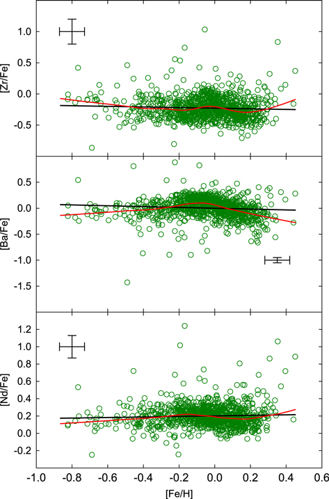
Figure 9. [Zr/Fe], [Ba/Fe], and [Nd/Fe] as a function of [Fe/H]. The solid black line is a linear fit to the data, while the red line is a LOESS smoothing. There are no believable trends in the data other than increased scatter relative to that seen in the α and Fe-peak elements. The error bars are the mean standard deviation of each species taken across the sample. See text for discussion.
Download figure:
Standard image High-resolution imageA primary point of interest in the s/r data is the behavior of Ba. It appears that [Ba/Fe] decreases once the [Fe/H] ratio goes above solar. LH07 found the same thing in their data and ascribed the effect to either non-LTE or line-formation problems. Both LH07 and this study used a maximum equivalent width cutoff of 20 nm to help control problems in inadequate line-formation modeling. Calculations show that non-LTE effects in Ba for more luminous stars (Andrievsky et al. 2013, 2014) are modest, contributing an uncertainty/non-LTE correction of about 0.1 dex in the Ba abundances. The primary uncertainty detected was inadequate line modeling (i.e., the Ba ii line cores go optically thick at very shallow continuum optical depths). The line strength cutoff applied here is well below the values found in the Cepheids considered in the non-LTE studies. The conclusion is that non-LTE is not the primary culprit in the Ba data for the giants. Because these are stronger lines, a more probable cause is that the equivalent widths are somewhat underestimated due to the Gaussian approximation missing the growing line wings. This possibility is given credence because a consideration of computed Ba ii profiles at 4950 K, log g = 2.5, and Vt = 1.5 km s−1 indicates that the Gaussian approximation underestimates the Voigt profile equivalent width of a true 20.0 pm line by 1.3 pm. While this difference is small, the line is saturated and the abundance needed to match the lesser equivalent width is 0.11 dex lower than that needed to match the Voigt profile value. Any underestimation in equivalent width will lead to potentially significant underabundances.
As a last point, the abundances here are overall in good agreement with those of LH07 and other works. Since the new data in no way contradicts previous analyses, there is no tension between the results of this study and the contention of Reddy et al. (2012, 2013) that field giants are the product of the breakup of open clusters. In fact, the cluster giants that are contained in this work are indistinguishable from the field giants in terms of their abundances.
4.4. Li, C, and O in Giants
The discussion of LH07 concerning lithium, carbon, and oxygen abundances in giants is still relevant today and their major points will be revisited briefly here.
4.4.1. Lithium
Lithium abundances have been determined in a range of local objects including dwarfs by Lambert & Reddy (2004) and Luck & Heiter (2006), as well as giants by Brown et al. (1989) and LH07. The base findings for the giants are that lithium is highly depleted with respect to its assumed initial value, and the depletion is a function of the effective temperature and mass. Recent studies of lithium in giants have focused on comparisons of thick and thin disk stars and the effects of rotation (Ramírez et al. 2012; Liu et al. 2014), with the result that thin disk giants are more lithium depleted than thick disk giants. There appears to be no dependence in giants of lithium on the macroturbulent or rotational velocity (LH07; Liu et al. 2014).
Theoretical predictions by Iben (1967a, 1967b) indicate that lithium should be diluted/depleted during the first giant branch by a factor of 60 at 3 M⊙, decreasing to a factor of 28 at 1 M⊙. However, recent work has shown that lithium abundance predictions in giants are subject to large numerical treatment uncertainties in thermohaline mixing (Lattanzio et al. 2015). While acknowledging that the theoretical predictions are uncertain, the currently available projected lithium dilutions/depletions correspond to decreases in abundance of 1.8–1.4 dex, relative to the (assumed constant) main sequence initial value. However, the surface lithium content of dwarfs is extremely variable (Lambert & Reddy 2004; Luck & Heiter 2006), spanning up to two orders of magnitude at any temperature/mass. While this makes the lithium content of any one star (giant or dwarf) impossible to predict under any evolutionary scheme, one can hopefully use overall trends in the data to test generic theoretical predictions.
The work of Lambert & Reddy indicates that the general astration level of lithium in dwarfs is independent of metallicity, but dependent upon mass. In Figure 10, we show their LTE abundance data (lithium versus mass), along with the G/K giant data of this study. The data shown in Figure 10 for the giants is from the LTE analysis. The non-LTE corrections from Lind et al. (2009) increase the lithium abundances by about 0.1 to 0.2 dex for both G/K giants and dwarfs. Figure 10 also shows the level of dilution predicted by standard evolution (a representative factor of 40). As apparent from the figure and pointed out by LH07, given the scatter in the dwarf lithium abundances and the mass-dependent astration, it is entirely possible that the bulk of giant lithium abundances are consistent with standard evolution. Because the dilution occurs/starts when the star becomes convective at the base of the first giant branch, the appropriate abundance to use for the dilution can be significantly below the local interstellar value of about 3.0–3.2 (as determined from the dwarfs themselves; see Lambert & Reddy). A detailed consideration of lithium abundances in giants may need additional dilution processes, but certainly not at the level one would need if the initial abundance were 3.0 dex or above.

Figure 10. Dwarf lithium abundances from Lambert & Reddy (2004) and giant lithium abundances from this work are shown vs. mass. The abundances for both groups assume LTE. The vertical arrows show the result of standard evolution in this mass range. See text for more discussion.
Download figure:
Standard image High-resolution imageFurther confounding the interpretation of the giant abundances is the "Li-dip," which is the observed decline in lithium abundance in open cluster dwarfs at a mass of about 1.3–1.4 M⊙ (Balachandran 1995). Later work has shown that the dip occurs at different temperatures/masses depending on the metallicity (François et al. 2013). However, the "Li-dip" is not an especially distinct feature in field dwarfs (Lambert & Reddy 2004; Luck & Heiter 2006), and so it is difficult to ascribe all of the variation in dwarf and giant lithium abundances to its presence.
In Figure 10, several stars show very high abundances of lithium: HR 7820, HR 8642, HD 188993, HD 9746, HD 95799, and HD 112127. All of these stars have lithium abundances in excess of 3.0 dex, with the last three stars in the super-Li (or Li-rich) list of Charbonnel & Balachandran (2000). The first three are stars in LH07 and all have lithium abundances consistent with the present values in that work. LH07 identified HR 7820 and HR 8642 as K giant super-Li stars. The evolutionary status assumed for a super-Li star is either that it is on the ascent to the first giant branch, or that it resides near the red-giant clump post first dredge-up. In either case, it will be well separated from the main sequence. This means that stars blueward of the clump, such as HD 188993, while having high Li abundances are not super-Li stars. HD 148317, which was not plotted in Figure 10, fails the culling process because it is too close to the main sequence. It shows a lithium abundance of 3.04 dex. The idea is that stars such as HD 188993 and HD 148317 have not yet undergone a strong mixing event and thus show their original lithium content. The status of these two stars will be considered further in the discussion of carbon and oxygen.
About 1% of normal K giants are super-Li stars (Charbonnel & Balachandran 2000). The question is what abundance level constitutes a super-Li star? Some of the stars listed by Charbonnel & Balachandran have lithium abundances as low as 1.5 dex. The number of stars having an abundance at that level or above in this study is 23, or slightly more than 2% of the sample. Note that these stars do not include any F giants near the main sequence or stars like HD 148317 and HD 188993. Thus it appears that this sample has too many super-Li stars. However, lithium abundances are very variable and it is certainly possible that a lithium abundance of 1.5–1.7 dex—dilution of a factor of 20–50—in a giant merely reflects standard evolution operating on the plateau local interstellar lithium abundance. If the lower abundance to consider as super-Li were taken to be 2.0 dex, this sample then has 15 total candidates.
Super-Li stars are "classified" according to their position in the HR diagram. In Figure 11, we see a group of these stars straddling the red-giant clump—the position of one of the two families of such objects (Charbonnel & Balachandran). The four stars, including HD 188993 blueward of the clump, may be from before the first dredge-up and thus have not diluted their surface lithium. Charbonnel & Balachandran gave a working hypothesis for the clump super-Li stars. The mechanism is an "extra" mixing that occurs at this position in the HR diagram between the convective envelope and the top of the H-burning shell. The mixing results in the production of 7Li, which is then convected to the surface. However, a trigger mechanism is still missing for the event. This scenario is complicated by the inconsistency in the theoretical lithium predictions found by Lattanzio et al. (2014). The takeaway from their study is that all theoretical lithium predictions should be viewed with caution.
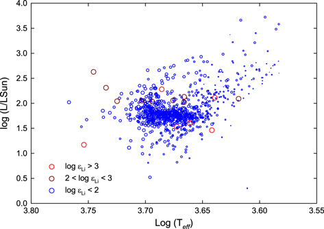
Figure 11. A bubble plot of lithium abundances in the clump region of the HR diagram. Symbol size reflects the lithium abundance: larger circles are higher abundances. The Li-rich stars found in the hotter regions may represent pre first dredge-up stars. The super-Li stars span the extent of the red-giant clump.
Download figure:
Standard image High-resolution image4.4.2. C and O
The abundances of carbon, nitrogen, and oxygen in K giants will reflect the effects of both galactic chemical evolution and stellar evolution. The properties of both galactic and stellar CNO evolution are well-known, having been studied numerous times (see, e.g., Lambert & Ries 1981; Gustafsson et al. 1999, LH07; Adamczak & Lambert 2014). The primary galactic evolution expectation is that the [O/Fe] (and [C/Fe]) ratio should rise with decreasing [Fe/H]. Stellar evolution will affect the carbon and nitrogen abundances—carbon will be converted to nitrogen with the sum C+N expected to remain constant. The anticipated carbon decrease is modest, perhaps up to 0.2 dex. Oxygen abundances are unchanged during the first dredge-up.
The relationship between [Fe/H] and [C/Fe], [O/Fe], and C/O is shown in Figure 12. As expected, both [C/Fe] and [O/Fe] increase with decreasing [Fe/H]. The C/O ratios are mostly subsolar, as projected based on the predictions of standard stellar evolution. Carbon is diluted/depleted because of the first dredge-up, while oxygen remains unaffected. Note that C/O is not independent of [Fe/H], but decreases, implying an enhancement of O relative to C in the more metal-poor stars. Our giant data is in accord with the C/O ratios found using the dwarf data of Luck & Heiter (2006). Their data gives solar C/O ratios at solar metallicity, with the C/O ratio declining toward lower [Fe/H] values, albeit with significant scatter. Gustafsson et al. (1999) also found this result in dwarfs. This implies that stellar evolution in this mass and metallicity range yields rather uniform results in the carbon dilution/depletion for the first dredge-up.
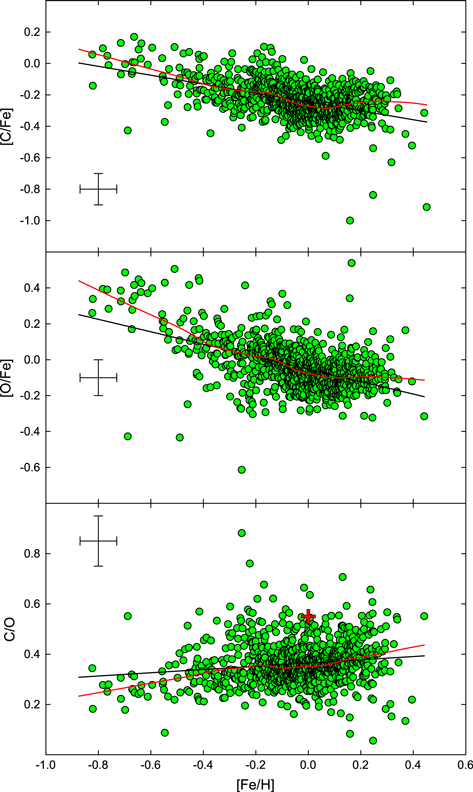
Figure 12. [C/Fe], [O/Fe], and C/O as a function of [Fe/H]. The trends seen here are well-known and result from the SNe Ia, producing relatively more iron as a function of time. The solar C/O ratio is indicated by the red cross in the bottom panel. These stars show the overall effects of standard galactic and stellar chemical evolution. The error bar in [Fe/H] is the mean standard deviation (±0.07) across the sample and the carbon and oxygen abundance uncertainty is estimated as ±0.1 from the synthesis and parameter uncertainties.
Download figure:
Standard image High-resolution imageThere are of order 50 C/O ratios at or slightly above the solar ratio in the current data. If these stars were actually dwarfs, one might expect their [C/Fe] ratio to be near zero, and they should have higher gravities relative to the mean of the sample. However, neither of these expectations are borne out. Perhaps the real question is why should a G/K giant be limited to a subsolar C/O ratio? The C/O ratio in local dwarfs spans a considerable range: 0.1 < C/O < 0.9 (Luck & Heiter 2006). The range seen in the G/K giants is consistent with those initial ratios coupled to standard stellar evolution, yielding a dilution/depletion of the surface carbon abundance by about 0.2 dex relative to the initial composition (Iben 1967a, 1967b; Schaller et al. 1992; Girardi et al. 2000).
LH07 pointed out an interesting result in their clump [C/Fe] abundances: They found that the blue side (i.e., hotter stars) in the clump showed lower [C/Fe] ratios than did the red-side. The difficulty was that an admixture of [Fe/H] ratios could give rise to a spurious result because [C/Fe] correlates with [Fe/H]. The current sample affords the possibility of exploring this effect further because there are more than 350 stars with [Fe/H] ratios between −0.1 and +0.1 dex that fall in the luminosity range 1.0 < log (L/L⊙) < 2.5. Figure 13 (top panel) shows the temperature-binned [C/Fe] ratios. Looking at the outermost points, we see that they differ in [C/Fe] by about 0.15 dex, with the blue edge having the lower abundance. Note that neither [O/Fe] or [Fe/H] show any dependence on temperature. There is an effect in the C/O ratio, but this is expected given the decrease in [C/Fe] and the lack of a variation in the [O/Fe] values against effective temperature.

Figure 13. Binned [C/Fe], [O/Fe], [Fe/H], and CO ratios as a function of temperature and mass. The stars have been selected to have −0.1 < [Fe/H] < 0.1 and 1.0 < log(L/L⊙) < 2.5. The increase in the [C/Fe] ratio toward cooler temperatures and lower mass indicates that the depth of mixing is a function of mass, which is an effect predicted by stellar evolution models. The error bar is one standard deviation around the mean value shown.
Download figure:
Standard image High-resolution image
Accepting the trend in [C/Fe] at face value, what could be the cause? The abundance ratios are plotted against mass in the bottom panel of Figure 13. Here we see that the [C/Fe] ratios of −0.3 to −0.4 are associated with higher mass stars (2.5–3.5 M⊙), whereas [C/Fe] increases to about −0.2 with decreasing mass. The obvious explanation is depth-dependent mixing as a function of mass: higher mass stars mix deeper, bringing more carbon deficient material to the surface than is the case in the lower mass stars. As mass correlates with age, a dependence exists between age and [C/Fe]—the strongest dilutions/depletions exist in the youngest stars. This is in accord both qualitatively and quantitatively with theoretical expectations (Iben 1967a, 1967b; Schaller et al. 1992; Girardi et al. 2000). More advanced stellar mixing/evolution schemes are available than the ones cited above. However, nitrogen abundance is needed to elaborate, and it is unavailable for most of the stars considered. Thus, the overall discussion will stop here. However, a few specific points do need further elaboration.
Figure 13 shows three stars that have very low [C/Fe] ratios. These stars must be akin to the weak G-band and/or the CN-stars discussed by Adamczak & Lambert (2013) and Luck (1991), respectively. Stars in these classes typically show carbon depletions up to 20 times larger than those found in normal giants; but as of now, there is no mechanism to explain them. The stars in this study that show such depletions are HR 6791, HR 40, and HR 1219. HR 6791 is a well-known example also included in both studies noted previously. The other two have not been mentioned in prior works on carbon-poor giants—HR 1219 and HR 40 are warmer objects, and have lower luminosities, placing them nearer the Main Sequence. The rotational/macroturbulent line broadening seen in both is of order 4 to 6 km s−1, making the lack of C i lines very obvious. Perhaps these stars are precursors to the more evolved post first giant branch weak G-band stars.
In the lithium discussion, two stars were identified with high Li contents: HD 188993 and HD 148317. Both stars are warmer and have higher gravities—about 5700 K and 3.5—and thus are likely G subgiants. Their carbon abundances are consistent with the idea that they have yet to ascend the first giant branch and undergo strong mixing: the [C/Fe] ratio in both is about +0.06. These two stars are likely on their redward pass toward the first giant branch.
As a last point, it is generally assumed that older stars are more metal-poor than younger stars, and that there is significant scatter within the age–metallicity relation. The idea of an age–metallicity relation is further complicated by the strong possibility that the stars will migrate during their lifetimes and end up far from their point of origin in radial distance from the galactic center (Sellwood & Binney 2002; Schönrich & Binney 2009). The difficulty with this scenario relative to the age–metallicity relation is that stars from different parts of the Galaxy should have different initial compositions, due to the galactic metallicity gradient (Luck & Lambert 2011). While this study was not designed to look at this problem, it is worth noting that the giant subset used to explore [C/Fe] in the red-giant clump (some 350 stars), has a total range in [Fe/H] of 0.2 dex centered on the solar value; but it has ages spanning more thatn 5 Gyr—from 0.5 to about 6 Gyr. There is little evidence for strong age–metallicity relation in the giants of the local region about the Sun.
5. CONCLUDING REMARKS
This study presents parameter and abundance data on more than 1130 giants in the local neighborhood. This is likely the largest high-resolution spectroscopic abundance study ever undertaken. The most striking result on parameters is the severe disagreement between the isochrone-mass-derived gravities and ionization-balance gravities. There is no accord currently available to rectify the difference. Astroseismology comes down on the side of the isochrone-mass-derived gravities, and then proceeds to attribute the difference to NLTE effects. However, the ability to attribute this difference to NLTE is disputed. One perhaps should worry about using 1D or 2D static model atmospheres to model an inherently dynamic spheroid.
In terms of the abundances, the local GK giants look much like the Sun—same total content with similar abundance ratios. Lithium, carbon, and oxygen abundances in the GK giants are substantially as predicted by standard stellar evolution. The lithium abundances are severely diluted, but once the "initial" dwarf abundances are taken into account, the dilution is most likely not substantially in excess of that predicted by standard evolutionary models. The oxygen abundances are unmodified from the initial value: that is, [O/Fe] = 0 when [Fe/H] is near 0. Carbon abundances are affected by CN processing and subsequent mixing during the first dredge-up. The mean [C/Fe] ratio in the sample is about −0.2 dex. A variation in the [C/Fe] ratio across the red-giant clump is identified as being due to mass-dependent mixing during the first giant branch. This result is discernible due to the large number of solar-metallicity (−0.1 < [Fe/H] < +0.1) giants in the sample. Effects of galactic chemical abundance are also present: [O/Fe] and [C/Fe] show their well-known dependence on [Fe/H].
The next step in this overall project will be to analyze a similarly sized sample of local FGK dwarfs designed to serve as an unevolved comparison sample.
I am grateful to a most conscientious referee whose comments substantially improved this paper. Financial support by Case Western Reserve University made possible the McDonald Observatory observations used in this work. The Sandiford echelle spectra used here are available through the FGK Spectral Library.2 This study is based in part on data obtained from the ESO Science Archive Facility under many request numbers. The ELODIE archive at Observatoire de Haute-Provence (OHP) also provided part of the spectroscopic data. The SIMBAD database—which is operated at CDS, Strasbourg, France, and satellite sites—and NASA's Astrophysics Data System Bibliographic Services were instrumental in this work.
Footnotes
- 1
IRAF is distributed by the National Optical Astronomy Observatories, which are operated by the Association of Universities for Research in Astronomy, Inc., under cooperative agreement with the National Science Foundation.
- 2