


ABSTRACT
The observed relation between supermassive black hole (SMBH) mass (M•) and bulge stellar velocity dispersion (σ*) is described by log M• = α + βlog(σ*/200 km s-1). As this relation has important implications for models of galaxy and SMBH formation and evolution, there continues to be great interest in adding to the M• catalog. The "sphere of influence" (ri) argument uses spatial resolution to exclude some M• estimates and pre-select additional galaxies for further SMBH studies. This Letter quantifies the effects of applying the ri argument to a population of galaxies and SMBHs that do not follow the M•–σ* relation. All galaxies with known values of σ*, closer than 100 Mpc, are given a random M• and selected when ri is spatially resolved. These random SMBHs produce a M•–σ* relation of α = 8.3 ± 0.2, β = 4.0 ± 0.3, consistent with observed values. Consequently, future proposed M• estimates should not be justified solely on the basis of resolving ri. This Letter shows that the observed M•–σ* relation may simply be a result of available spatial resolution. However, it also implies that the observed M•–σ* relation defines an upper limit. This potentially provides valuable new insight into the processes of galaxy and SMBH formation and evolution.
Export citation and abstract BibTeX RIS
1. INTRODUCTION
There has been a growing database of direct supermassive black hole (SMBH) mass (M•) estimates from the centers of nearby galactic bulges (e.g., Graham 2008b). While the limits of our current abilities to significantly expand this database may have been reached (Batcheldor & Koekemoer 2009), the last decade has seen a wealth of M• estimates that have increased the SMBH catalog from 13 or 26 (Ferrarese & Merritt 2000; Gebhardt et al. 2000) to ∼70 (Graham 2008b; Hu 2008; Gültekin et al. 2009). An intense interest in populating the SMBH database was sparked by observed correlations between M• and fundamental properties of their host bulges (e.g., Kormendy & Richstone 1995; Magorrian et al. 1998; Ferrarese & Merritt 2000; Gebhardt et al. 2000; Graham et al. 2001; Ferrarese 2002; Marconi & Hunt 2003; Baes et al. 2003; Häring & Rix 2004; Pizzella et al. 2005). These M• scaling relations have generated numerous theoretical investigations (e.g., Ciotti & van Albada 2001; Adams et al. 2003; Cattaneo et al. 2005; Robertson et al. 2006) and have possibly added valuable limits to evolutionary models (e.g., Heckman et al. 2004; Wyithe & Loeb 2005; Treu et al. 2007; Ciotti 2009).
The degree to which an SMBH's sphere of influence, ri, is resolved has been used as a quality measure for M• estimates (Ferrarese 2002; Marconi & Hunt 2003; Valluri et al. 2004). The only method available to a priori determine if a M• estimate can be made is to assume ri = GM•/σ2* (Peebles 1972). However, to calculate ri in galaxies with known σ*, M• is estimated using the M•–σ* relation given by log M• = α + βlog(σ*/200 km s-1), where α = 8.1–8.2 and β = 3.7–4.9. The observed scatter,  , is 0.4 dex (Novak et al. 2006; Graham & Li 2009). Following this, Figure 1 demonstrates where ri will be resolved, given a spatial resolution of ℜ = 0
 1. A value of ℜ = 01 is used here as that is the typical FWHM of the Hubble Space Telescope (HST) point-spread function (PSF). To date, HST has been responsible for most M• estimates.
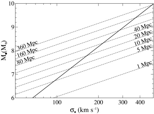
Figure 1. Observable M•–σ* plane at discrete distances based on ℜ = 01 and α = 8.2, β = 4.6 (solid line). In areas above the dashed distance lines, ri will be resolved if the galaxy with the given σ* hosts the given SMBH.
Download figure:
Standard image High-resolution imageFerrarese & Ford (2005, FF05) discussed the limited abilities of HST to resolve ri, and Gültekin et al. (2009, G09) found the M•–σ* relation to be biased when applying the ri argument. The influence of ri cuts on the M•–σ* relation is continued in this Letter with two significant advances. First, a sample of all galaxies with a known σ* (<100 Mpc) is used. It is important to only use these galaxies as there are no σ* = 400 km s−1 galaxies at 1 Mpc, for example. Second, random M• estimates are applied to each galaxy, i.e., no galaxy is assumed to intrinsically fall on the M•–σ* relation. This ensures no pre-selection of galaxies that lie on the M•–σ* relation. Throughout, a distinction is made between the observed M•–σ* relation (published values) and the observable M•–σ* relation (the relation that can be fitted using the data simulated here).
2. METHODS AND RESULTS
In short, these simulations take a galaxy with a known σ* and distance, assign a M•, then calculate ri. The ri argument is then applied; if ri is unresolved the galaxy is removed from the sample (the low-mass cut). If the assigned M• generates a galaxy that lies above the observed M•–σ* relation, it is also removed from the sample (the high-mass cut). The observable M•–σ* relation is then fit to the remaining galaxies using a Levenberg–Marquardt least-squares add-on to IDL.
A SQL search of the Hyperleda1 catalog was performed (Paturel et al. 2003). All galaxies with a kinematical distance modulus less than 35.0 (100 Mpc, assuming H0 = 70 km s-1 Mpc-1) were found. Of the 49,740 galaxies returned, 2518 have published values of σ*. The incompleteness of this sample, due to difficulties in measuring σ* in faint galaxies, is noted. Values of ri (in arcsec) were then calculated for each galaxy by assigning a M•.
In the first cases, the low-mass cut was made by applying ℜ = 01 to represent the HST PSF. However, several values of ℜ are applied later. The high-mass cuts were then made by considering the observed distribution of galaxies in the M•–σ* plane; there is a clear absence of over-massive SMBHs, i.e., there are no σ* = 50 km s−1 dwarf spheroids in the Local Group with M• ∼109M☉. Such a nearby over-massive SMBH population would have been detected, and therefore it is assumed that these objects do not exist. Galaxies selected for the high-mass cuts were determined by assigning a scatter ( = 0.4 dex) and upper limits to the M•–σ* relation, (M•–σ*)u. Galaxies with ri > rmax(Mmax) were removed from the sample, where ![$M_{\rm max} = [\epsilon + 10^{\alpha _u}(\sigma /200{\rm \ km\ s^{-1}})^{\beta _u}]M_\odot$](https://content.cld.iop.org/journals/2041-8205/711/2/L108/revision1/apjl337349ieqn1.gif) .
.
Each galaxy was first assigned 90 separate values of M• using a step size of 100.1 from 101.0M☉ to 1010.0M☉. In this case, the high-mass cut was made by applying the αu = 8.1, βu = 4.2 relation of G09 and the αu = 8.2, βu = 4.9 relation of FF05. Figure 2 shows the distribution of observable galaxies in the M•–σ* plane assuming every galaxy within 100 Mpc can host any M• and that ℜ = 01. The fit to this sample (red line) is α = 8.4, β = 3.5.
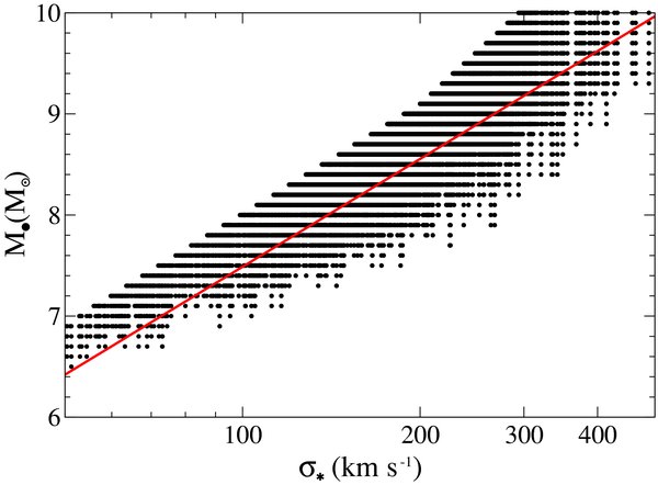
Figure 2. Simulated M•–σ* data points (black circles) based on a ℜ = 01 criteria. This demonstrates the observable region of the M•–σ* plane with the assumption that there is no M•–σ* relation. The fitted M•–σ* relation (red line) is α = 8.4, β = 3.5.
Download figure:
Standard image High-resolution imageHowever, galaxies host single (or binary) SMBHs, therefore it is shrewd to assign each galaxy a single (uniformly sampled) random value for M• in the range 101–1010M☉. The distribution of observable galaxies in the M•–σ* plane using a random sample of M• is shown in Figure 3 using the red open circles. In this case, the low-mass cut was made using ℜ = 01, and the high-mass cut was made using the (M•–σ*)u relation of αu = 8.1, βu = 4.2, = 0.4 (G09). The M•–σ* relation fit to these observable galaxies (red line) is αu = 8.3, βu = 4.1, = 0.2 dex. An observable M•–σ* relation of αu = 8.3, βu = 4.6, = 0.4 dex is found using the high-mass (M•–σ*)u relation of FF05. Figure 3 also shows all observed galaxies based on the combined catalogs of Graham (2008b), Hu (2008), and G09. No distinction is made between "good" and "bad" M• estimates, or differences in quoted σ*; all estimates are plotted (143 total).
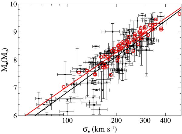
Figure 3. Distribution of observable galaxies from a random distribution of M• (red circles) using the (M•–σ*)u relation of G09. All present estimates of M• and σ* are shown as filled black circles, with uncertainties. The fit to the observable galaxies (red circles and line) is α = 8.3, β = 4.1.
Download figure:
Standard image High-resolution imageThe similarity between the M•–σ* distribution of observable random mass SMBHs and observed SMBHs masses is striking. However, as this result derives from a single random sampling of M•, it represents a single possible observable M•–σ* relation. If galaxies intrinsically have random M• values, then the range of observable SMBHs could have a distribution given by the distribution in Figure 2. Therefore, 50 separate random M• samplings were then made for each galaxy, and in each case a fit to the observable M•–σ* relation was performed. In addition, as the previously used value of ℜ = 01 only applies to HST observations, the analysis was repeated for a range of ri lower cutoffs. Finally, as the high-mass cuts may not actually be defined by the G09 and FF05 fits, values of αu from 7.8 to 8.7 (in 0.1 steps) and βu from 3.6 to 5.4 (in 0.2 steps) were used to create an addition 100 individual (M•–σ*)u cutoffs. The mean values of α, β and , derived by applying these different ℜ criteria, and from using these variable upper limits, are presented in Table 1.
Table 1. Effects of the ri Cutoff from Averaged Random M• Distributions
| ℜ | Observed α | Observed β | Observed |
|---|---|---|---|
| (Zero Point) | (Slope) | (Scatter) | |
| Variable Upper Cutoffs | |||
| 005 |
8.25 ± 0.17 | 3.80 ± 0.33 | 0.41 dex |
| 010 |
8.25 ± 0.21 | 3.90 ± 0.34 | 0.27 dex |
| 015 |
8.25 ± 0.23 | 3.93 ± 0.34 | 0.22 dex |
| 020 |
8.25 ± 0.27 | 4.01 ± 0.38 | 0.18 dex |
| Fixed Upper Cutoffs | |||
| 005 |
8.44 ± 0.03 | 3.93 ± 0.23 | 1.82 dex |
| 010 |
8.57 ± 0.02 | 4.02 ± 0.21 | 1.22 dex |
| 015 |
8.64 ± 0.02 | 4.03 ± 0.25 | 0.97 dex |
| 020 |
8.68 ± 0.03 | 4.07 ± 0.32 | 0.85 dex |
Notes. Average results from applying variable and fixed M•–σ* upper limits to 50 random M• samples. A fixed upper limit of αu = 8.7 and βu = 5.0 was used based on the upper-limit fit in Figure 4. If there was no intrinsic M•–σ* relation, these are the values of the M•–σ* relation that would be observed using the different spatial resolutions listed.
Download table as: ASCIITypeset image
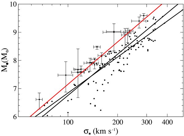
Table 1 has several notable features. First, as ℜ rises falls. This is expected because the range of observable SMBHs decreases with larger values of ℜ. Second, the slope (β) remains consistent. Finally, in the case of the variable upper limits, the zero point (α) remains constant and is consistent with the mid-value of the (M•–σ*)u limits imposed on the sample. To test whether these values of α are a consequence of the high-mass cut conditions, the analysis was repeated using αu limits of 7.0 and 8.8 (in 0.2 steps). Applying a ℜ = 01 low-mass cut, an observable relation with α = 8.0 ± 0.5 was found. Again, the values of α are consistent with the mid-value of the imposed limits. However, an estimate of the observed (M•–σ*)u relation can be made. The observed SMBH sample in Figure 3 was used to define an upper limit by fitting all observed SMBHs that fall above the FF05 and G09 relations, and above = 0.4. The fit to these over-massive SMBHs produce an upper limit of αu = 8.7, βu = 5.0 (Figure 4). This (M•–σ*)u fit was then applied to 50 random values of M• in each galaxy, and the observable M•–σ* relations were then fitted in each case. The average of these fits are also presented in Table 1. In this case, the fitted values of α and β are consistent with the variable upper limits, but the values of are significantly larger. This is expected, as these fits were applied to data that had the maximum range in the M•–σ* plane due to the high observed values of αu and βu.
Figure 4. Fitting the observed (M•–σ*)u relation. Filled black circles are the M•–σ* points, those with error bars are the points used for the upper fit (shown in red). The red upper-limit fit is α = 8.7, β = 5.0. The two solid black lines are the observed G09 and FF05 fits.
Download figure:
Standard image High-resolution image
3. DISCUSSIONS
In summary, as a result of applying the ri argument, a M•–σ* relation consistent with observed values (α ≈ 8, β ≈ 4, ≈ 0.3 dex) can be fitted to a sample of galaxies that contain random mass SMBHs, and as a consequence do not follow a M•–σ* relation. The ri argument removes low-mass SMBHs where ri would not be resolved, and high-mass SMBHs where ri should have been resolved if such a population were present. Therefore, for scaling relations to be of value in constraining galaxy evolution models, M• estimates must not be solely proposed on the basis of critically resolving values of ri derived from σ*.
It is unlikely that an intrinsic M•–σ* relation has been observed as a result of critically sampling ri in the M•–σ* plane, and it will be some time until we are able to sample a significant area rightward of the observed M•–σ* relation (e.g., FF05; Batcheldor & Koekemoer 2009). Therefore, it is clear that caution must be used in the application of the observed M•–σ* relation until this issue can be resolved.
The possibility of there being no tight intrinsic M•–σ* relation, and that the distribution of observed galaxies in the M•–σ* plane determine an upper limit only, is now discussed. As the same M• estimates are used to define the other M• scaling relations, this also implies that all observed scaling relations are upper limits. There are a number of questions arising from this possibility, beginning with the most fundamental. Why do observed SMBHs fall on the M•–σ* relation? There are several SMBHs with such high quality M• estimates (Sgr A*, NGC 4258, M87), that there clearly is a relation between M• and σ* in some galaxies. However, the M•–σ* plane has been increasingly populated with less certain M• estimates that have potentially been included on the assumption that ri is spatially resolved, i.e., that they follow a previously estimated M•–σ* relation defined by higher quality M• estimates. In these cases, as the simulations presented here show, an observed M•–σ* relation will arise simply as a result of the ri selection effect, even if M• is randomly distributed within galaxies.
Does a population of under-massive SMBHs exist, and have they been detected? If the M•–σ* relation is an upper limit, then there should be galaxies that host low-mass SMBHs, as suggested by simulations (Vittorini et al. 2005; Volonteri 2007). Indeed, both the simulations presented here, and the observations plotted in Figure 3, show that under-massive SMBHs can be, and have been, detected. Some notable cases are that of NGC 4435 (Coccato et al. 2006), a sample of barred galaxies (Graham 2008a), and narrow-line Seyfert 1 galaxies (Mathur & Grupe 2005). In fact, the evidence to suggest the presence of under-massive SMBHs is not matched by any evidence for a significant population of over-massive SMBHs leftward of the observed M•–σ* relation.
It is important to note some intricacies with the two dominant techniques for measuring M• (stellar and gas dynamics). In the case of stellar dynamics, there are systematics to the models that may allow a large range of M• in a given bulge (Valluri et al. 2004). In the case of gas dynamics, it is unclear what the inclination of the nuclear gas disk may be (e.g., Marconi et al. 2003). Both methods allow the potential for many of the current M• estimates to in fact be upper limits, i.e., the true M•–σ* plane may have a large distribution of under-massive SMBHs. Therefore, under-massive SMBHs may have been observed, their mass overestimated, and their impact overlooked.
All SMBH models allow stringent upper limits to be placed on M• (e.g., Sarzi et al. 2002; Beifiori et al. 2009). However, these M• upper limits will also be dependent on the available spatial resolution. Any kinematical data will have two velocity points spatially separated on a scale of ℜ. An upper limit to M• is estimated by including an increasing dark mass until the derived model becomes inconsistent with the data, i.e., a higher upper limit to M• will be estimated using a lower ℜ. There are still important constraints that can be added to the M•–σ* plane from estimates of M• upper limits, however, as upper limits that fall below the observed M•–σ* relation provide the same evidence for under-massive SMBHs as would a tightly constrained low-mass M•. At present, most M• upper limits are based on data derived from gas dynamics. Consequently, these limits generally fall above the observed M•–σ* relation due to unknown amounts of line broadening from non-gravitational processes, and uncertainty in the inclination of the nuclear gas disks.
If the M•–σ* relation represents an upper limit in the M•–σ* plane, then what is this limit? In Section 2, an upper limit of αu = 8.7, βu = 5.0 was found based on the distribution of observed SMBHs leftward of the observed M•–σ* relation. This is likely a good approximation to the (M•–σ*)u limit as there are no reports of a steeper relation. However, this estimate does not include the potential over-massive SMBHs from the upper limits calculated by Beifiori et al. (2009). Including these limits to the upper limit sample gives values of αu = 8.8, βu = 3.9 to (M•–σ*)u. As expected, due to the addition of SMBH limits at lower M•, this (M•–σ*)u limit is more shallow with a higher zero point. Including these limits at the lower M• end of the M•–σ* plane addresses, in part, a limitation of the sample used here. As already noted, the σ* catalog used here is likely incomplete due to the difficulty of measuring σ* in faint galaxies at greater distances. In addition, the σ* catalog likely contains inhomogeneous measurements that may not translate from bulge to bulge.
What are the consequences to galaxy evolution models if there is only a (M•–σ*)u relation? First, galaxies will no longer be required to obey the M•–σ* relation, and could host a SMBH with any M• below (M•–σ*)u. Models that include feedback from the SMBH to the galaxy will then need to be carefully reconsidered. While the SMBH will undoubtedly have some influence on a portion of the host galaxy, it would not need to affect large-scale properties; evolution of the SMBH would be a result of host galaxy evolution. An upper limit in the M•–σ* plane would also represent the pinnacle of SMBH evolution as a function of σ*, in which galaxies evolve up to the (M•–σ*)u limit. A signature of such a scenario could be a cosmic variation in (the scatter would increase with redshift) and an observed M•–σ* relation that does not exceed (M•–σ*)u. If the distribution of M• is random within bulges, then when compared with the local observed M•–σ* relation, M• estimates from higher redshift could fall to the left or the right. Treu et al. (2007) find a population of z = 0.36 Seyfert 1 galaxies that lie above the local observed M•–σ* relation by Δlog σ = 0.13, Δlog M• = 0.54, but this population still lies below the (M•–σ*)u limit estimated here. Finally, if SMBHs can reside anywhere below the (M•–σ*)u limit, then the local black hole mass function may have been overestimated. This would relax the observation that merging is not important and that SMBH growth is dominated by accretion (e.g., Marconi et al. 2004). This potentially allows anti-hierarchical SMBH growth to no longer present problems for hierarchical galaxy formation models.
The use of the HyperLeda database (http://leda.univ-lyon1.fr) is acknowledged. D.B. thanks Alessandro Marconi, David Merritt, and Andy Robinson for useful discussions. Support for this work was provided by proposal number HST-AR-10935.01 awarded by NASA through a grant from the Space Telescope Science Institute, which is operated by the Association of Universities for Research in Astronomy, Inc., under NASA contract NAS5-26555.