Generalization and network design strategies

Источник: Yan LeCun - Generalization and Network Design Strategies. 1989. - 9 pages Generalization and Network Design Strategies Y. le Cun Department of Computer Science University of Toronto Technical Report CRG-TR-89-4 June 1989 Send requests to: The CRG technical report secretary Department of Computer Science University of Toronto 10 Kings College Road Toronto M5S 1A4 CANADA INTERNET: carol@ai.toronto.edu UUCP: uunet!utai!carol BITNET: carol@utorgpu This work has been supported by a grant from the Fyssen foundation, and a grant from the Sloan foundation to Geoffrey Hinton . The author wishes to thank Geoff Hinton, Mike Mozer , Sue Becker and Steve Nowlan for helpful discussions, and John Denker and Larry Jackel for useful comments. The Neural Network simulator SN is the result of a collaboratiOn between Leon-Yves Bottou and the author. Y. le Cun 's present address is Room 4G-332 , AT&T Bell Laboratories, Crawfords Corner Rd, Holmdel, NJ 07733. Y. Le Cun. GeneralizatiOn and network design strategies. Technical Report CRG-TR-89-4, University of Toronto Connectionist Research Group, June 1989. a shorter version was published in Pfeifer, Schreter, Fogelman and Steels (eds) 'Connectionism in perspective', Elsevier 1989. Generalization and Network Design Strategies Yann le Cun * Department of Computer Science, University of Toronto Toronto, Ontario, M5S 1A4. CANADA. Abstract An interestmg property of connectiomst systems is their ability to learn from examples. Although most recent work in the field concentrates on reducing learning times, the most important feature of a learning machine is its generalization performance. It is usually accepted that good generalization performance on real-world problems cannot be achieved unless some a pnon knowledge about the task is butlt Into the system. Back-propagation networks provide a way of specifymg such knowledge by imposing constraints both on the architecture of the network and on its weights. In general, such constramts can be considered as particular transformations of the parameter space Building a constramed network for image recogmtton appears to be a feasible task. We descnbe a small handwritten digit recogmtion problem and show that, even though the problem is linearly separable, single layer networks exhibit poor generalizatton performance. Multtlayer constrained networks perform very well on this task when orgamzed in a hierarchical structure with shift invariant feature detectors. These results confirm the idea that minimizing the number of free parameters in the network enhances generalization. 1 Introduction Connect10mst architectures have drawn considerable attention m recent years because of the1r interestmg learnmg abihtles Among the numerous learnmg algorithms that have been proposed for complex connectiomst networks, • Present address: Room 4G-332, AT&T Bell Laboratories, Crawfords Corner Rd, Holmdel, NJ 07733. 1 Back-Propagatwn (BP) 1s probably the most widespread. BP was proposed in (Rumelhart et al, 1986), but had been developed before by several independent groups m d1fferent contexts and for d1fferent purposes (Bryson and Ho, 1969, Werbos, 1974, le Cun, 1985; Parker, 1985; le Cun, 1986) Reference (Bryson and Ho, 1969) was m the framework of optimal control and system identification, and one could argue that the bas1c 1dea behind BP had been used m optimal control long before 1ts apphcatwn to machme learning was considered (le Cun, 1988) Two performance measures should be considered when testing a learning algonthm learning speed and generahzatwn performance Generalization is the mam property that should be sought, 1t determmes the amount of data needed to tram the system such that a correct response 1s produced when presented a patterns outside of the trammg set. We will see that learnmg speed and generahzation are closely related . Although various successful applications of BP have been described in the literature, the conditions m which good generalization performance can be obtamed are not understood. Cons1dermg BP as a general learning rule that can be used as a black box for a wide vanety of problems 1s, of course, Wishful thmkmg Although some moderate sized problems can be solved using unstructured networks, we cannot expect an unstructured network to generalize correctly on every problem. The main pomt of th1s paper 1s to show that good generahzat10n performance can be obtamed 1f some a przorz knowledge about the task 1s bu1lt mto the network. Although in the general case specifymg such knowledge may be difficult , 1t appears feas1ble on some h1ghly regular tasks such as image and speech recogm tion. Tallonng the network architecture to the task can be thought of as a way of reducmg the s1ze of the space of poss1ble functwns that the network can generate, without overly reducmg 1ts computatwnal power Theoretical studies (Denker et al , 1987) (Patarnello and Carnevah, 1987) have shown that the likehhood of correct generahzat10n dep ends on the size of the hypothesis space (total number of networks bemg considered), the s1ze of the solutiOn space (set of networks that g1ve good generalizatiOn) , and the number of trauung examples If the hypothesis space IS too large and/ or the number of tranmg examples IS too small, then there will be a vast number of networks wh1ch are consistent w1th the trauung data, only a small proportwn of wluch will hem the true solutwn space, so poor generalization IS to be expected Conversely, 1f good generalizatiOn IS reqmred, when the generality of the architecture 1s mcreased, the number of trammg examples must also be mcreased. Specifically, the reqmred number of examples scales like the loganthm of the number of functiOns that the network architecture can Implement 2 An Illuminating analogy can be drawn between BP learning and curve fitting. When usmg a curve model (say a polynomial) with lots of parameters compared to the number of points, the fitted curve w1ll closely model the training data but will not be hkely to accurately represent new data. On the other hand, 1f the number of parameters in the model is small, the model will not necessanly represent the trainmg data but w1ll be more likely to capture the regularity of the data and extrapolate (or interpolate) correctly. When the data is not too noisy, the optimal choice is the mimmum size model that represents the data. A common-sense rule msp1red by this analogy tells us to minimize the number of free parameters m the network to increase the likelihood of correct generahzatwn But th1s must be done without reducing the size of the network to the pomt where it can no longer compute the desired function. A good compromise becomes poss1ble when some knowledge about the task is available, but the pnce to pay 1s an mcreased effort in the design of the architecture. 2 Weight Space Transformation Reducmg the number of free parameters m a network does not necessarily Imply reducmg the s1ze of the network Such techmques as weight sharing, descnbed in (Rumelhart et al , 1986) for the so-called T-C problem, can be used to reduce the number of free parameters while preservmg the s1ze of the network and spec1fymg some symmetnes that the problem may have. In fact, three mam techmques can be used to build a reduced s1ze network. The first techmque 1s problem-mdependent and cons1sts m dynamically deletmg "useless" connectiOns dunng trammg Th1s can be done by addmg a term m the cost functiOn that penalizes b1g networks w1th many parameters Several authors have descnbed such schemes, usually Implemented as a non-proportional we1ght decay (Rumelhart, personnal communication 1988), (Chauvm, 1989, Hanson and Pratt, 1989), or usmg "gatmg coefficients" (Mozer and Smolensky, 1989) GeneralizatiOn performance has been reported to increase s1gmficantly on small problems Two drawbacks of this techmque are that It requires a fine tumng of the "prumng" coefficient to avo1d catastrophic effects, and also that the convergence 1s s1gmficantly slowed down 2.1 Weight Sharing The second techmque IS we1ght shanng Weight sharmg consists m havmg several connectwns (Imks) be controlled by a smgle parameter (weight) We1ght sharmg can be mterpreted as 1mposmg equality constramts among the connectiOn strengths. An mterestmg feature of weight sharmg IS that 1t can be 3 Figure 1. We1ght Space Transformation. implemented with very httle computat10nal overhead. Weight sharmg is a very general paradigm that can be used to descnbe so-called Time Delay Neural Networks used for speech recogmtion (Wa1bel et al. , 1988, Bottou, 1988), timeunfolded recurrent networks, or sh1ft-mvanant feature extractors. The expenmental results presented m this paper make extensive use of weight sharing. 2.2 General Weight Space Transformations The third techmque, which really IS a generahzat10n of weight shanng, 1s called weight-space transformation (WST) (le Cun, 1988) WST is based on the fact that the search performed by the learnmg procedure need not be done in the space of connection strengths, but can be done m any parameter space that JS SUitable for the task Th1s can be ach1eved prov1ded that the connect10ns strengths can be computed from the parameters through a given transformat10n, and provided that the Jacobian matnx of th1s transformatiOn IS known, so that we are able to compute the partials of the cost funct10n with respect to the para meters The gradient of the cost functwn With resp ect to the parameters IS then Just the product of the Jacobian matnx of the transformation by the gradient w1th respect to the connect10n strengths. The situatiOn 1s depicted on figure 1 2.2.1 WST to improve learning speed Several types of WST can be defined, not only for reducmg the s1ze of the parameter space, but also for speedmg up the learnmg 4 Although the followmg example IS quite difficult to Implement in practice, It gives an Idea about how WST can accelerate learning. Let us assume that the cost functwn C mmimized by the learnmg procedure is purely quadratic w r. t the connectwn strengths W In other words, C is of the form where W IS the vector of connection strengths, H the Hessian matrix (the matnx of second derivatives) which will be assumed positive definite Then the surfaces of equal cost are hyperparaboloids centered around the optimal solutwn Performing steepest descent m this space will be ineffi.etent If the eigenvalues of H have wide vanatwns In this case the paraboloids of equal cost are very elongated formmg a steep ravine The learning time is known to depend heavily on the ratio of the largest to the smallest eigenvalue. The larger this ratio, the more elongated the paraboloids, and the slower the convergence. Let us denote A the diagonalized verswn of H, and Q the unitary matnx formed by the (orthonormal) eigenvectors of H, we have H = QT AQ. Now, let :E be the diagonal matnx whose elements are the square root of the elements of A, then H can be rewntten asH= QTr.r.Q We can now rewrite the expression for C(W) in the followmg way Usmg the notatwn U = EQW we obtain In the space of U, the steepest descent search will be tnvial smce the Hessian matnx Is equal to the Identity and the surfaces of equal cost are hyper-spheres The steepest descent direction points m the direction of the solution and lS the shortest path to the solutwn Perfect learning can be achieved in one smgle Iteratwn If Q and :E are known accurately. The transformation for obtammg the connectwn strengths W from the parameters U is simply Durmg learnmg, the path followed by U in U space is a straight line, as well as the path followed by W m W space This algonthm is known as Newton's algonthm, but IS usually expressed directly m W space. Performmg steepest descent m U space IS equivalent to usmg Newton's algonthm m W space. Of course m practice tlus kmd of WST IS unrealistic since the size of the Hessian matnx IS huge (number of connectwns squared), and smce It IS qUite 5 expensive to estimate and diagonahze Moreover, the cost function IS usually not quadratic m connectiOn space, which may cause the Hessian matnx to be non positive, non defimte, and may cause 1t to vary w1th W Nevertheless, some approximatiOns can be made wluch make these Ideas 1mplementable (le Cun, 1987, Becker and le Cun, 1988) 2.2.2 WST and generalization The WST just described IS an example of problem-zndependent WST, Other kinds of WST which are problem-dependent can be devised . Building such transformation requires a fair amount of knowledge about the problem as well as a reasonable guess about what an optimal network solutiOn for th1s problem could be Fmdmg WST that Improve generahzatwn usually amounts to reducing the s1ze of the parameter space. In the followmg sectwns we describe an example where simple WST such as weight sharmg have been used to Improve generalIzation 3 An example: A Small Digit Recognition Problem The following experimental results are presented to Illustrate the strategies that can be used to design a network for a particular problem The problem descnbed here IS m no way a real world application but 1s sufficient for our purpose The mtermed1ate size of the database makes the problem non-tnvial, but also allows for extensive tests of learnmg speed and generalizatiOn performance 3.1 Description of the Problem The database IS composed of 480 examples of numerals represented as 16 pixels by 16 pixels binary Images 12 example of each of the 10 digits were handdrawn by a single person on a 16 by 13 bitmap usmg a mouse Each Image was then used to generate 4 examples by puttmg the origmal1mage m 4 consecutlVe honzontal positions on a 16 by 16 b1tmap The trammg set was then formed by choosmg 32 examples of each class at random among the complete set of 480 Images the remammg 16 examples of each class were used as the test set Thus, the trammg set contamed 320 Images. and the test set contamed 160 Images On figure 2 are represented some of the trammg examples 6 Figure 2. Some examples of input patterns. 3.2 Experimental Setup All simulations were performed usmg the BP simulator SN (Bottou and le Cun, 1988) Each umt m the network computes a dot product between 1ts input vector and 1ts weight vector This weighted sum, denoted a, for unit i, is then passed through a sigmoid squashmg functiOn to produce the state of unit i, denoted by x, x, = f(a,) The squashmg functiOn IS a scaled hyperbolic tangent: J(a) = A tanh Sa where A IS the amplitude of the function and S determmes its slope at the ongm, and f IS an odd functiOn, with horizontal asymptotes +A and -A Symmetnc functions are believed to yield faster convergence, although the learmng can become extremely slow If the weights are too small The cause of tlus problem IS that the ongm of weight space is a stable point for the learnmg dynamics , and , although it is a saddle pomt, it is attractive m almost all duectwns For our simulatiOns, we use A= 1. 7159 and S = ｾﾷ＠ with this choice of pa1ameters, the equaht1es /(1) 1 and f( -1) -1 are satisfied The ratwnale behind th1s IS that the overall gam of the squashmg transformatiOn Is around 1 m normal operatmg conditions, and the interpretation of the state of the network IS Simplified Moreover, the absolute value of the second derivative = = 7 off IS a maximum at +1 and -1, which Improves the convergence at the end of the learnmg session. Before trainmg, the weights are mitiahzed with random values usmg a Uniform distribution between -2.4/ F, and 2.4/ F, where F, is the number of inputs (fan-m) of the unit which the connectiOn belongs to 1 . The reason for dividing by the fan-m IS that we would like the initial standard deviation of the wetghted sums to be m the same range for each unit, and to fall within the normal operatmg regwn of the s1gmo1d If the Initial weights are too small, the gradients are very small and the learnmg Is slow, 1f they are too large, the sigm01ds are saturated and the gradient is also very small The standard deviation of the weighted sum scales hke the square root of the number of inputs when the inputs are mdependent, and it scales hnearly with the number of mputs 1f the mputs are highly correlated. We chose to assume the second hypothesis smce some units receive highly correlated signals The output cost functiOn IS the usual mean squared error- where P IS the number of patterns, Dop IS the desired state for output unit o when pattern p IS presented on the input. Xop IS the state of output Unit o when pattern p IS presented. It is worth pomtmg out that the target values for the output units are well w1thm the range of the sigmoid This prevents the weights from growmg mdefinitely and prevents the output units from operatmg m the flat spot of the sigmOid. AdditiOnally, smce the second derivative of the sigmOid IS maximum near the target values, the curvature of the error functiOn around the solutiOn IS maximized and the convergence speed during the final phase of the learnmg process is Improved Durmg each learning experiment, the patterns were presented in a constant order, and the training set was repeated 30 times. The weights were updated after each presentation of a smgle pattern according to the so-called stochastic gradtent or "on-line" procedure Each learnmg experiment was performed 10 times with different initial conditiOns All experiments were done both usmg standard gradient descent and a special verswn of Newton's algonthm that uses a positive, diagonal approximation of the Hessian matrix (le Cun, 1987, Becker and le Cun, 1988) All experiments were done usmg a special verswn of Newton's algonthm that uses a positive, diagonal approximatiOn of the Hessian matnx (le Cun, 1987, Becker and le Cun, 1988) Tlus algorithm IS not believed to brmg a tremendous 1 smce several connectwns share a we1ght th1s rule could be difficult to apply, but m our case, all connections sharing a same weight belong to umts w1th 1dentical fan-ms 8 mcrease m learnmg speed but it converges reliably w1thout requiring extens1ve adJustments of the learnmg parameters At each learning 1terat10n a particular weight Uk (that can control several connect10n strengths) 1s updated according to the followmg rule Uk +- Uk L + fk (s,;)EVk fJC Ｍｾﾭ UWs; where C 1s the cost function, w, 1 is the connection strength from unit j to unit IS the set of unit mdex pairs (i,J) such that the connection strength w, 1 IS controlled by the we1ght Uk. The step s1ze fk is not constant but 1s funct10n of the curvature of the cost functwn along the axis Uk. The expressiOn for fk is· i, Vk where .A and J.l are constant and hkk is a running estimate of the second denvatlve of the cost functwn C with respect to Uk. The terms hkk are the diagonal terms of the Hess1an matnx of C w1th respect to the parameters Uk. The larger hkkl the smaller the we1ght update The parameter J.l prevents the step size from becommg too large when the second derivat1ve is small, very much like the "model-trust" methods used in non-linear optlm1zation. Special actions must taken when the second derivat1ve is negative to prevent the weight vector from gomg uphill Each hkk 1s updated according to the following rule: where 1 IS a small constant wh1ch controls the length of the window on which the average 1s taken The term 8 2 C is given by: 1 jaw; fJ2C fJ2C - - - --x2 ow?. - oa 2 J '1 ' where x 1 1s the state of umt J and 8 Cfaa; is the second derivative of the cost functwn w1th respect to the total input to umt i (denoted a,) These second deuvatlves are computed by a back-propagatiOn procedure sim1lar to the one used for the first denvat1ves (le Cun, 1987)· 2 2 8 C "'ii""2 ua, 2 2 2 8 C = !'( a, ) "'"" ｾ＠ w ks "'ii""2 - f "( a, ) ｾ＠ fJC k uak ux, The first term on the nght hand s1de of the equation is always posit1ve, while the second term, mvolvmg the second denvat1ve of the squashmg functiOn J, 9 can be negative. For the simulatwns, we used an approximation to the above expression that gives positive estimates by simply neglectmg the second term: fJ2C a, 7f2 = f I 2 ｾ＠ (a,) ＠ｾ 2 fJ2C wkl{j2 k ak This corresponds to the well-known Levenberg-Marquardt approximatwn used for non-hnear regresswn (see for example (Press et al., 1988)). This procedure has several interestmg advantages over standard non-linear optimizatwn techniques such as BFGS or conjugate gradient. First, it can be used m conjunction With the stochastic update (after each pattern presentatwn) smce a line search IS not reqmred. Second, It makes use of the analytzcal expresswn of the diagonal Hessian, standard quasi-Newton methods estzmate the second order properties of the error surface Third, the scaling laws are much better than With the BFGS method that reqmres to store an estimate of the full Hessian matnx 2 In this paper, we only report the results obtamed through this pseudoNewton algonthm smce they were consistently better than the one obtamed through standard gradient descent The mput layer of all networks were 16 by 16 binary images, and their output layer was composed of 10 units, one per class. An output configuratwn was considered correct If the most-activated unit corresponded to the correct class. In the followmg, when talking about layered networks, we Will refer to the number of layers of modifiable weights. Thus, a network With one hidden layer IS referred to as a two-layer network 3.3 Net-1: A Single Layer Network The simplest network that can be tested on this problem IS a smgle layer, fully connected network with 10 sigmoid output units (2570 weights mcludmg the biases) Such a network has successfully learned the trammg set, which means that the problem is hnearly separable But, even though the trammg set can be learned perfectly, the generalizatwn performance IS disappomtmg. between 80% and 72% dependmg on when the learnmg IS stopped (see curve 1 on figure 3). Interestmgly, the performance on the test set reaches a maximum qmte early durmg trammg and goes down afterwards This over-trammg phenomenon has been reported by many authors The analys1s of this phenomenon IS outside the scope of this paper. When observmg the weight vectors of the output umts , 1t becomes obvwus that the network can do nothmg but develop a set of matched filters tuned to match an "average pattern" formed by superimposmg 2 Recent developments such as Nocedal's "lmuted storage BFGS" may alleviate this problem 10 100 .. 90 .- . - . ... net1 . - . -I . ---------------1-!--- net2 / , . ,_..,.. _.......;::.::.:,.,_..,...................................... --·-l·-···· net3 ....... " r:: 80 0 net4 .... ｾ＠ t: 0 () net5 70 ｾ＠ 60 0 5 10 15 20 training epochs 25 30 Figure 3 GeneralizatiOn performance vs traming time for 5 network architectures Net-1 smgle layer, Net-2: 12 hidden units fully connected, Net-3. 2 hidden layers locally connected, N et-4· 2 hidden layers, locally connected With constramts, N et-5· 2 hidden layers, local connections, two levels of constraints all the trammg examples Despite its relatJVely large number of parameters, such a system cannot possibly generalize correctly except in trivial situations, and certamly not when the input patterns are slightly translated. The classification IS essentially based on the computatiOn of a weighted overlap between the input pattern and the "average prototype" 3.4 Net-2: A Two-Layer, Fully Connected Network The second step IS to insert a hidden layer between the input and the output. The network has 12 hidden units , fully connected both to the mput and the output There IS a total of 3240 weights mcluding the biases. Predictably, this network can also learn perfectly the trammg set m a few epochs 3 (between 7 and 15) The generalizatiOn performance IS better than with the previOus 3 The word epoch IS used to designate an enhre pass through the tram1ng set, wruch m our case Is equivalent to 320 pattern presentatiOns 11 10 10 4x4 8x8 16x16 16x16 16x16 Figure 4: three network architectures Net-1, Net-2 and Net-3 network and reaches 87% after only 6 epochs (see figure 3). A very slight overlearnmg effect is also observed, but Its amplitude IS much smaller than with the prevwus network. It IS mteresting to note that the standard devmtion on the generalization performance IS s1gmficantly larger than with the first network. This an mdication that the network IS largely underdetermined, and the number of solutions that are consistent with the trammg set is large. Unfortunately, these vanous solutions do not give eqmvalent results on the test set, thereby explaming the large variations m generalizatiOn performance. From this result, it is qmte clear that this network IS too big (or has too many degrees of freedom) 3.5 Net-3: A Locally Connected, 3-Layer Network Since reducmg the size of the network will also reduce Its generality, some knowledge about the task Will be necessary m order to preserve the network's abihty to solve the problem A simple solutiOn to our over-parameterization problem can be found if we remember that the network should recogmze Images. Classical work m visual pattern recogmtion have demonstrated the advantage of extractmg local features and combmmg them to form higher order features We can easily bmld this knowledge mto the network by forcmg the hidden units to only combine local sources of mformatwn. The architecture comprises two hidden layers named H1 and H2. The first hidden layer, H1, IS a 2-dimenswnal array of Size 8 by 8. Each unit in H1 takes Its mputs from 9 umts on the mput plane situated in a 3 by 3 square neighborhood. For umts in layer H1 that are 12 one umt apart, their receptrve fields (in the input layer) are two prxels apart Thus, the receptive fields of two nerghbouring hidden units overlap by one row or one column. Because of this two-to-one undersampling in each directwn, the mformatwn IS compacted by a factor of 4 going from the mput to Hl. Layer H2 is a 4 by 4 plane, thus, a similar two-to-one undersampling occurs gomg from layer H1 to H2, but the receptive fields are now 5 by 5. H2 is fully connected to the 10 output units. The network has 1226 connections (see figure 4) The performance is slightly better than with Net-2: 88.5%, but is obtained at a consrderably lower computational cost since Net-3 is almost 3 times smaller than N et-2. Also note that the standard deviation on the performance of N et-3 is smaller than for Net-2. This is thought to mean that the hypothesrs space for N et-3 (the space of possible functwns rt can implement) is much smaller than for Net-2 3.6 Net-4: A Constrained Network One of the major problems of Image recogmtion, even as simple as the one we consider m thrs work, rs that distmctrve features of an object can appear at vanous locatiOns on the input Image. Therefore it seems useful to have a set feature detectors that can detect a particular mstance of a feature anywhere on the mput plane. Since the preczse location of a feature is not relevant to the classrficatwn, we can afford to loose some positiOn information in the process. Nevertheless, an approxzmate posrtion information must be preserved in order to allow for the next levels to detect higher order features. DetectiOn of feature at any location on the input can be easrly done usmg werght sharmg. The first hrdden layer can be composed of several planes that we wrll call feature maps All umts m a plane share the same set of werghts, thereby detectmg the same feature at different locations. Since the exact posrtion of the feature IS not Important, the feature maps need not be as large as the input An mterestmg srde effect of this techmque rs that rt reduces the number of free werghts m the network by a large amount. The arclutecture of Net-4 rs very srmrlar to Net-3 and also has two hrdden layers The first hidden layer rs composed of two 8 by 8 feature maps. Each umt m a feature map takes mput on a 3 by 3 neighborhood on the mput plane For umts Ill a feature map that are one unit apart, therr receptrve fields in the mput layer are two prxels apart. Thus, as with Net-3 the input Image rs undersampled The mam difference with Net-3 is that all umts in a feature map share the same set of 9 werghts (but each of them has an mdependent bras) The undersamplmg techmque serves two purposes The first is to keep 13 10 10 4x4 ｌＭＮｊＱＧＬＺｾ＠ .....ＮｷＭｾ＠ 4x4x4 8x8x2 8x8x2 16x16 16x16 F1gure 5 two network architectures with shared weights: Net-4 and N et-5 the s1ze of the network w1thin reasonable hm1ts The second 1s to ensure that some locat10n information 1s discarded durmg the feature detectwn Even though the feature detectors are sh1ft mvariant , the operatwn they collectlvely perform is not. When the input 1mage 1s shifted, the output of the feature maps lS also shifted, but is otherwise left almost unchanged. Because of the two-to-one undersampling, when the shift of the input is small, the output of the feature maps is not shifted, but merely slightly distorted . As m the previous network, the second hidden layer is a 4 by 4 plane w1th 5 by 5 local receptive fields and no we1ght sharmg. The output is fully connected to the second hidden layer and has, of course, 10 umts. The network has 2266 connectwns but only 1132 (free) we1ghts (see figure 5) The generalizatwn performance of th1s network JUmps to 94%, mdicating that bmlt-m shift mvanant features are qmte useful for this task . This result also md1cates that, desp1te the very small number of mdependent we1ghts, the computational power of the network lS mcreased. 3.7 Net-5: A Network with Hierarchical Feature Extractors The same 1dea can be pushed further , leadmg to a hierarch1cal structure Wlth several levels of constramed feature maps The architecture of Net-5 is very similar to the one of N et-4, except that the second Iudden layer H2 has been replaced by four feature maps each of which 1s a 4 by 4 plane. Umts m these feature maps have 5 by 5 receptive fields in the 14 first hidden layer. Agam, all units m a feature map share the same set of 25 weights and have mdependent biases. And again, the two-to-one undersampling occurs between the first and the second hidden layer. The network has 5194 connectwn but only 1060 free parameters, the smallest number of all networks described m this paper (see figure 5). The generalization performance is 98.4% (100% generalization was obtained durmg two of the ten runs) and increases extremely quickly at the beginning of learnmg. This suggests that usmg several levels of constrained feature maps is a big help for shift invariance. 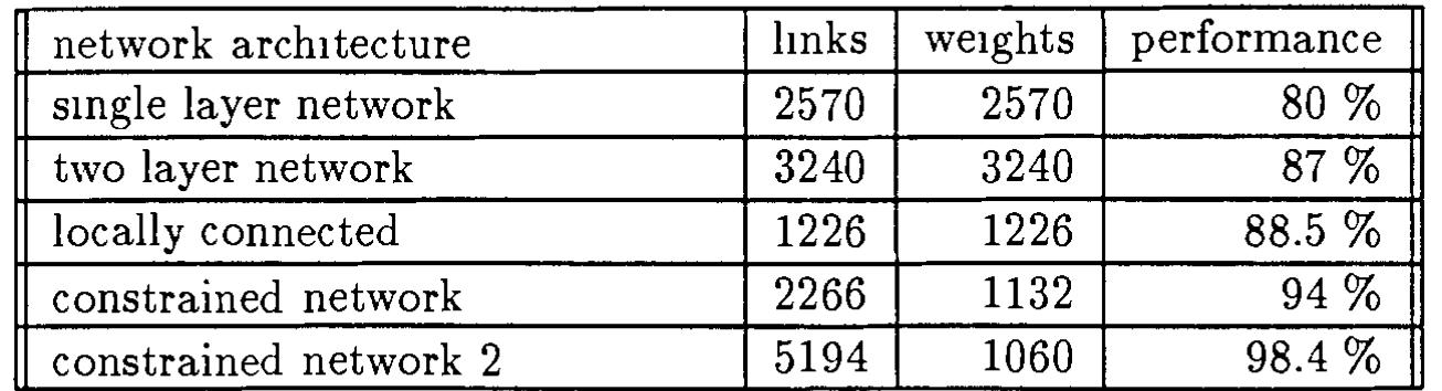4 Discussion The results are summanzed on table 1. As expected, the generahzation performance goes up as the number of free parameters in the network goes down and as the amount of built-in knowledge goes up. A noticeable exception to this rule is the result given by the singlelayer network and the two-layer, fully connected network. Even though the two layer net has more parameters, the generalization performance is significantly better One explanation could be that the one-layer network cannot classify the whole set (trammg plus testing) correctly, but experiments show that It can. We see two other possible explanatwns. The first one is that some knowledge is ImphCitly put by msertmg a hidden layer: we tell the system that the problem IS not first order. the second one IS that the efficiency of the learning procedure (as defined m (Denker et al., 1987)) IS better with a two layer net than with a one layer net, meanmg that more information is extracted from each example With the former . This is highly speculative and should be investigated further. 4.1 Tradeoff Between Speed, Generality and Generalization Computer scientists know that storage space, computation time and generahty of the code can be exchanged when designing a program to solve a particular problem For example, a program that computes a trigonometric function can use a senes expanswn, or a lookup table. the latter uses more memory than the former but IS faster. Usmg properties of trigonometric functions, the same code (or table) can be used to compute several functions, but usually results in some loss m efficiency. The same kind of exchange exists for learning machines. It 1s tnvial to des1gn a machme that learns very qmckly, does not generalize, and requires an enormous amount of hardware In fact this learnmg machine has already 15 lmks 2570 3240 1226 2266 5194 network architecture smgle layer network two layer network locally connected constrained network constrained network 2 we1ghts 2570 3240 1226 1132 1060 performance 80% 87% 88.5% 94% 98.4% Table 1 GeneralizatiOn performance for 5 network architectures. N et-1. smgle layer; Net-2: 12 hidden units fully connected; Net-3 2 hidden layers locally connected; Net-4: 2 hidden layers, locally connected with constramts; N et-5· 2 h1dden layers, local connections, two levels of constramts. Performance on training set is 100% for all networks been built and is called a Random Access Memory On the other hand, a back-propagation network 4 takes longer to train but is expected to generalize. Unfortunately, as shown m (Denker et al., 1987), generalization can be obtamed only at the pnce of generahty 4.2 On-Line Update vs Batch Update All s1mulatwns descnbed in this paper were performed using the so-called "online" or "stochastic" version of back-propagatiOn where the we1ghts are updated after each pattern, as opposed to the "batch" verswn where the weights are updated after the gradients have been accumulated over the whole trammg set. Expenment show that stochastic update is far supenor to batch update when there IS some redundancy m the data. In fact stochastic update must be better when a certain level of generahzatwn is expected. Let us take an example where the trammg database is composed of two cop1es of the same subset. Then accumulatmg the gradient over the whole set would cause redundant computations to be performed Stochastic gradient does not have this problem. This 1dea can be generalized to traming sets where there exist no prec1se repet1t10n of the same pattern but where some redundancy 1s present. 4.3 Conclusion vVe showed an example where constrammg the network architecture Improves both learnmg speed and generahzatwn performance dramatically Tins 1s re4 unless It IS designed to emulate a RAM 16 ally not surpnsmg but it Is more easily said than done. However, we have demonstrated that It can be done in at least one case, image recogmtion, using a hierarchy of shift mvariant local feature detectors. These techniques can be easily extended (and have been) to other domams such as speech recogm tion. Complex software tools with advanced user mterfaces for network description and simulatiOn control are required in order to solve a real application. Several network structures must be tried before an acceptable one is found and a quick feedback on the peformance is critical. We are just beginmng to collect the tools and understand the principles which can help us to deszgn a network for a particular task. Designing a network for a real problem Will require a Sigmficant amount of engineering, which the availability of powerful learnmg algorithms will hopefully keep to a bare mimmum Acknowledgments This work has been supported by a grant from the Fyssen foundation, and a grant from the Sloan foundatiOn to Geoffrey Hinton. The author wishes to thank Geoff Hmton, Mike Mozer, Sue Becker and Steve Nowlan for helpful discussiOns, and John Denker and Larry Jackel for useful comments. The Neural Network simulator SN is the result of a collaboratiOn between Leon-Yves Bottou and the author. References Becker, S and le Cun, Y (1988). Improving the convergence ofback-propagatwn learnmg with second-order methods. Technical Report CRG-TR-88-5, University of Toronto Connectwmst Research Group. Bottou, L-Y (1988) Master's thesis, EHEI, Universite de Pans 5. Bottou, L.-Y and le Cun, Y. (1988). Sn: A simulator for connectionist models. In Proceedzngs of NeuroNzmes 88, Nimes, France. Bryson, A and Ho , Y (1969) . Applzed Optzmal Control Blaisdell Publishmg Co Chauvm, Y (1989) A back-propagation algorithm with optimal use of hidden umts In Touretzky, D., editor, Advances zn Neural Informatzon Processzng Systems Morgan Kaufmann. 17 Denker, J., Schwartz, D., Wittner, B , Solla, S. A., Howard, R., Jackel, L., and Hopfield, J. ( 1987) Large automatic learning, rule extraction and generalization. Complex Systems, 1:877-922. Hanson, S. J. and Pratt, L. Y (1989) . Some comparisons of constramts for mmImal network construction with back-propagatiOn. In Touretzky, D., editor, Advances zn Neural Informatzon Processzng Systems. Morgan Kaufmann. le Cun, Y (1985). A learning scheme for asymmetric threshold networks. In Proceedzngs of Cognztzva 85, pages 599-604, Pans, France le Cun, Y (1986). Learnmg processes m an asymmetric threshold network. In Bienenstock, E., Fogelman-Souhe, F., and Weisbuch, G., editors, Dzsordered systems and bzologzcal organzzatzon, pages 233-240, Les Houches, France Sprmger-Verlag le Cun, Y. (1987). Modeles Connexzonnzstes de l'Apprentzssage. PhD thesis, Umversite Pierre et Mane Cune, Pans, France le Cun, Y. (1988). A theoretical framework for back-propagation. In Touretzky, D, Hinton, G., and SeJnowski, T., editors, Proceedzngs of the 1988 Connectzomst Models Summer School, pages 21-28, Cl\IU , Pittsburgh, Pa. Morgan Kaufmann. Mozer, M. C and Smolensky, P (1989) Skeletomzation: A techmque for trimmmg the fat from a network vm relevance assessment. In Touretzky, D., editor, Advances zn Neural Informatzon Processzng Systems. Morgan Kaufmann. Parker, D B. (1985). Learmng-logic. Technical report, TR-47, Sloan School of Management, MIT, Cambndge, Mass. Patarnello, S. and Carnevali, P (1987). Learning networks of neurons with boolean logic Europhyszcs Letters, 4( 4).503-508 Press, W H , Flannery, B. P., A., T . S. , and T., V. W . (1988) Reczpes Cambridge University Press, Cambndge. Numencal Rumelhart, D. E., Hinton, G E., and Williams, R . J. (1986) Learnmg mternal representatwns by error propagatwn. In Parallel dzstrzbuted processzng. Exploratzons zn the mzcrostructure of cognztzon, volume I Bradford Books, Cambndge, MA. 18 Waibel, A, Hanazawa, T., Hinton, G., Shikano, K., and Lang, K. (1988). Phoneme recogmtwn using time-delay neural networks. IEEE Transactzons on Acoustzcs, Speech and Szgnal Processzng. Werbos, P. (1974). Beyond Regresszon. Phd thesis, Harvard Umvers1ty. 19